Advanced plots and inference

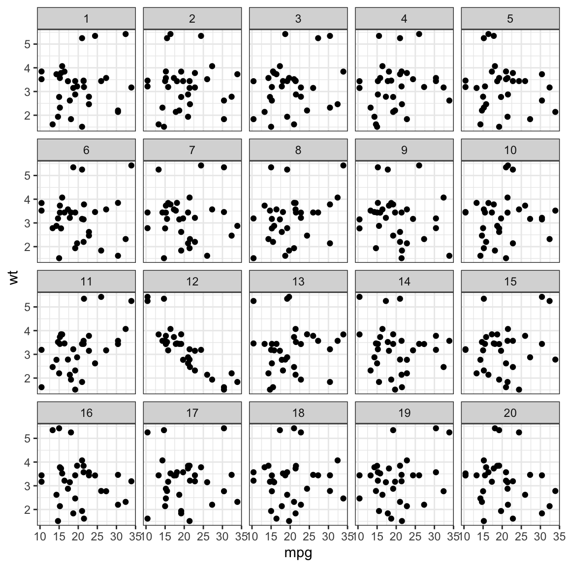
SISBID 2025
https://github.com/dicook/SISBID

Tidy data and random variables

• Tidy data mirrors elementary statistics
• Tabular form puts variables in columns and observations in rows
• Not all tabular data is in this form
• In this form, we can think about \(X_1 \sim N(0,1), ~~X_2 \sim \text{Exp}(1) ...\)

\[\begin{align}X &= \left[ \begin{array}{rrrr} X_1 & X_2 & ... & X_p \end{array} \right] \\ &= \left[ \begin{array}{rrrr} X_{11} & X_{12} & ... & X_{1p} \\ X_{21} & X_{22} & ... & X_{2p} \\ \vdots & \vdots & \ddots& \vdots \\ X_{n1} & X_{n2} & ... & X_{np} \end{array} \right]\end{align}\]

Grammar of graphics and statistics

• A statistic is a function on the values of items in a sample, e.g. for \(n\) iid random variates \(\bar{X}_1=\displaystyle\sum_{i=1}^n X_{i1}\), \(s_1^2=\displaystyle\frac{1}{n-1}\displaystyle\sum_{i=1}^n(X_{i1}-\bar{X}_1)^2\)
• We study the behaviour of the statistic over all possible samples of size \(n\).
• The grammar of graphics is the mapping of (random) variables to graphical elements, making plots of data into statistics

What is inference?

Inferring that what we see in the data at hand holds more broadly in life, society and the world.

Why do we need it for graphics?

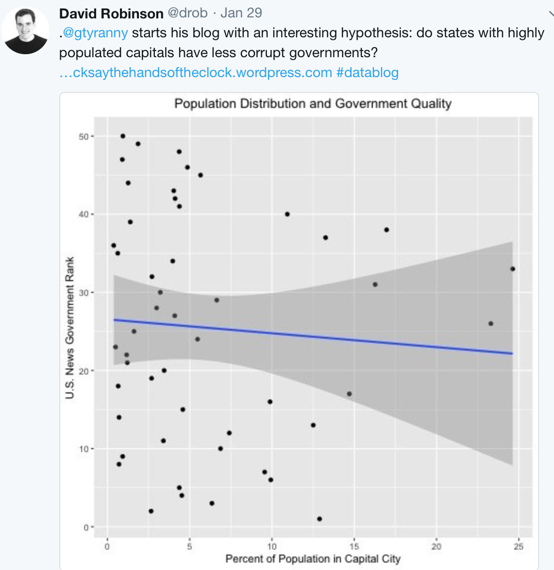
Here’s an example tweeted by David Robinson based on an analysis in Tick Tock blog by Graham Tierney

Source

From the blog: > I ran linear regressions of government rank on the percentage of each state’s population living in the capital city, state population (in 100,000s), and state GDP (in $100,000s)…. The coefficient is not significant for any regression at the traditional 5% level.

• A simple scatterplot of the two variables of interest.
• A slight negative slope is observed, but it does not look very large.
• There are a lot of states whose capitals are less than 5% of the total population.
• The two outliers are Hawaii (government rank 33 and capital population 25%) and Arizona (government rank 26 and capital population 23%).
• Without those two the downward trend (an improvement in ranking) would be much stronger.

… I’m not convinced that the lack of significance is itself significant.

To do statistical inference

You need a:

• statistic computed from the data
• null and alternative hypothesis
• reference distribution on which to measure the statistic
  • if it is extreme on this scale, reject the null

Inference with data plots

You need a:

• plot description provided by the grammar (a statistic)
  • This implies one or more null hypotheses
• null generating mechanism, e.g. permutation, simulation from a distribution or model
• visual evaluation: is one plot in the array different?

Some examples

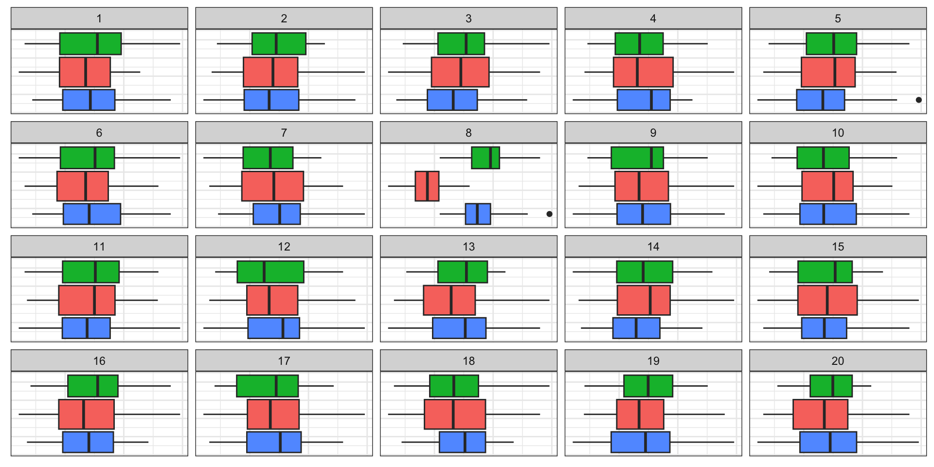
Here are several plot descriptions.
What would be the null hypothesis in each?

Which plot definition would best match
\(H_0:\) there is no difference in the distribution between the groups?

A - doesn’t show by group, so not useful. Would allow testing association between x1, x2 across groups. B - could be useful to show differences in mean on (x1, x2) by cl C - might allow testing whether distribution of x1 is symmetric D - Might show differences in distribution for x1

Some examples

Here are several null hypotheses.
What type of plot would you use to test each?

1. \(H_0:\) no association between x1 and x2
2. \(H_0:\) no difference between levels of cl
3. \(H_0:\) the distribution of x1 is XXX
4. \(H_0:\) no difference in the distribution of x1 b/w levels of cl

1. Scatterplot of x = x1, y = x2
2. Scatterplot of x = x1, y= x2, color = cl
3. Histogram of x1
4. violin plot of x1 with different colors

Let’s do it

# Make a lineup of mtcars data
# 20 plots, one data, 19 nulls
# Which one is different?
set.seed(20190709)
library(ggplot2)
ggplot(
  lineup(
    null_permute('mpg'), 
    mtcars), 
  aes(mpg, wt)
) +
  geom_point() +
  facet_wrap(~ .sample)

Example from the nullabor package. The data plot is embedded randomly in a field of null plots, this is a lineup. Can you see which one is different?

When you run the example yourself, you get a decrypt code line, that you run after deciding on a plot to print the location of the data plot amongst the nulls.

• plot is a scatterplot, null hypothesis is there is no association between the two variables mapped to the x, y axes
• null generating mechanism: permutation

Lineup

Mix the data plot
into a field of null plots

Which plot is different?

Null-generating mechanisms

• Permutation: randomizing the order of one of the variables breaks association, but keeps marginal distributions the same
• Simulation: from a given distribution, or model. Assumption is that the data comes from that model.

Evaluation

• Compute \(p\)-value
• Power \(=\) signal strength

p-values

• \(K\) independent observers
• \(x\) individuals pick the data plot from \(m\) plots

Assuming that all plots in a lineup are equally likely to be selected,

\[P(X\geq x) = \sum_{i=x}^{K} \binom{K}{i} \left(\frac{1}{m}\right)^i\left(\frac{m-1}{m}\right)^{K-i}\]

p-values

\[P(X\geq x) = \sum_{i=x}^{K} \binom{K}{i} \left(\frac{1}{m}\right)^i\left(\frac{m-1}{m}\right)^{K-i}\]

This is a Binomial model

For \(x=4\) picks, \(K=17\) observers, \(m=20\) plots

     x simulated       binom
[1,] 4    0.0202 0.008800605

p-values

But… some null plots are more visually salient!

p-values

Introduce a parameter \(\alpha\): visual salience of null plot dist

\[\begin{align}P(X \geq x) = &\sum_{i = x}^{K} \binom{K}{x} \frac{1}{B(\alpha, (m-1)\alpha)}\times \\ &B(x+\alpha, K-x+(m-1)\alpha),\end{align}\]

where \(B(.,.)\) is the Beta function.

This is a Beta-Binomial mixture model

p-values

• Large \(\alpha\): several null plots are ‘interesting’
• \(\alpha \approx 0.15\): 1 or 2 null plots are interesting enough to get some picks

Computing p-values with \(\alpha\):

alpha = 0.01 alpha = 0.15    alpha = 1 
  0.03397441   0.25942593   0.47220162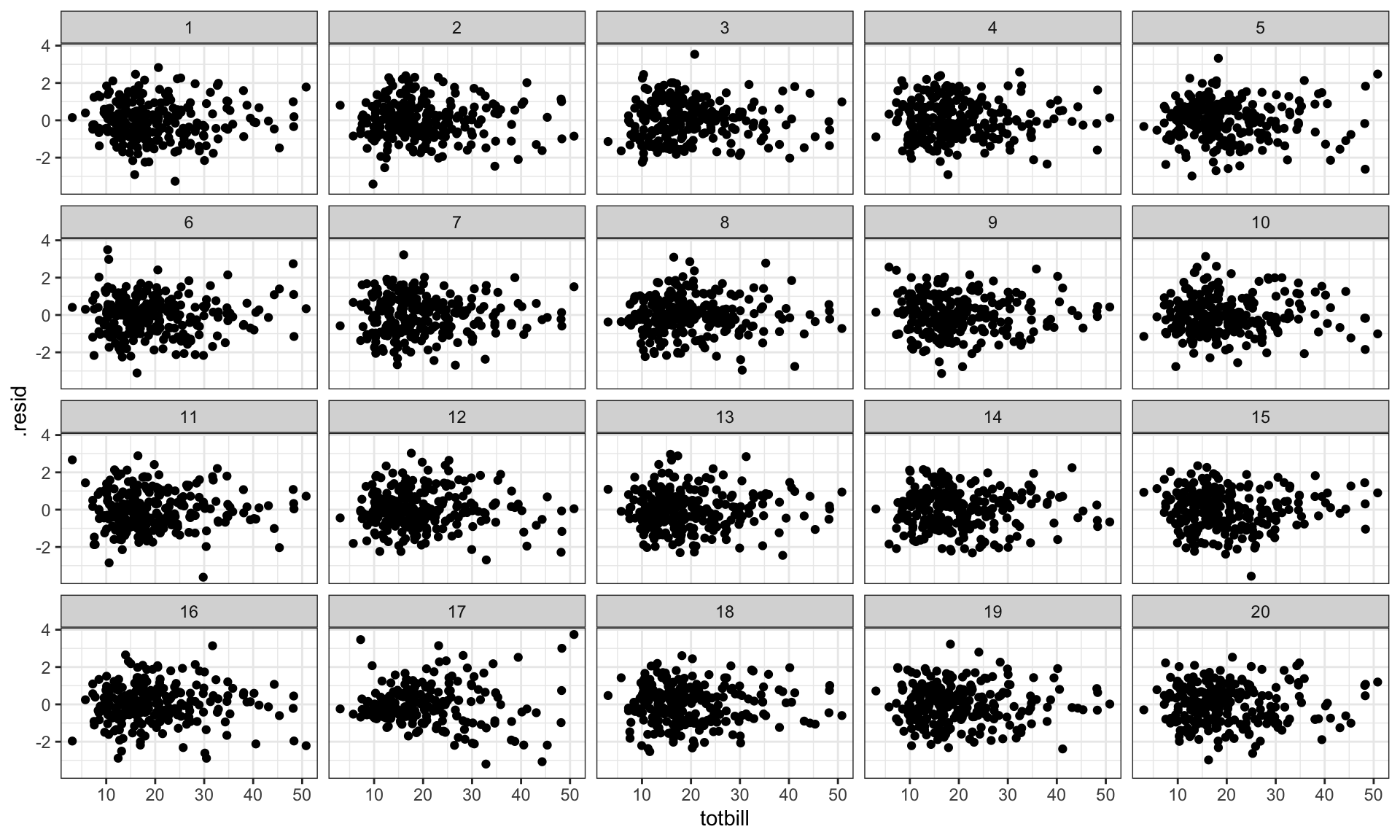 

Goodness-of-fit & residuals

• plot is a residual vs fitted scatterplot
• null hypothesis is no association between the two statistics
• null generating mechanism: residual rotation

Goodness-of-fit & residuals

Assessing temporal dependence

• line plot: \(H_0\) is there is no temporal trend
• nulls generated via simulation from a time series model

Assessing temporal dependence

ggplot(l, aes(x=date, y=rate)) + 
  geom_line() +
  facet_wrap(~.sample, 
             scales="free_y") +
  theme(axis.text = 
          element_blank()) +
  xlab("") + ylab("")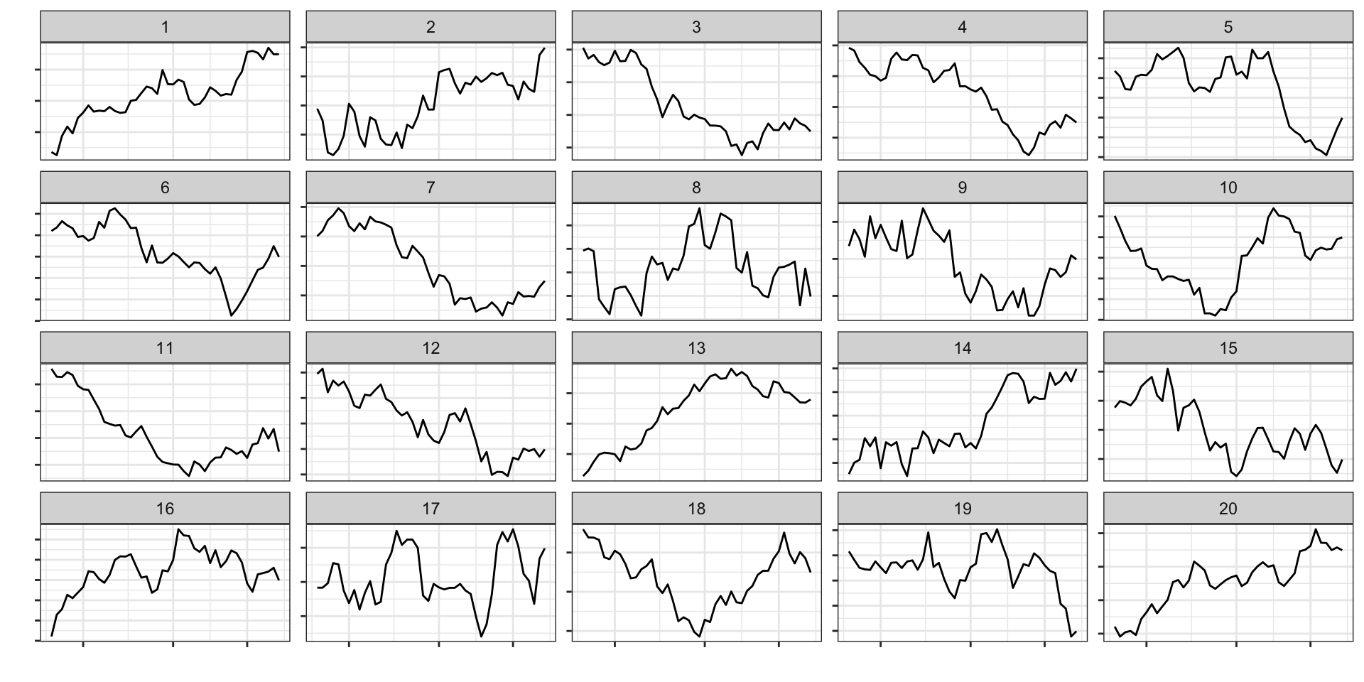

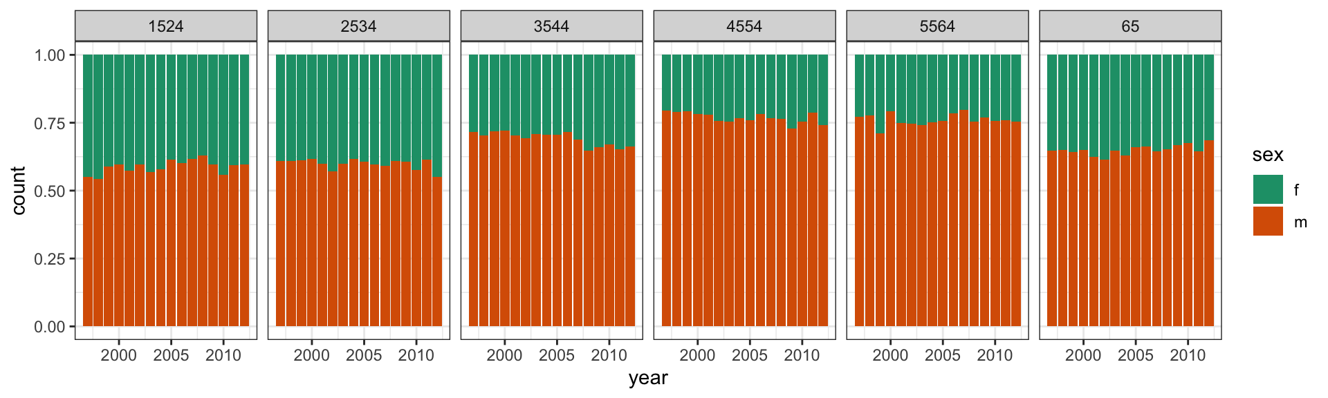
Let’s talk TB

Earlier:

• Across all ages, and years, the proportion of males having TB is higher than females
• These proportions tend to be higher in the middle age groups, for all years.
• Relatively similar proportions occur across years.

Null hypothesis

Plot count against year, separately for each age group, coloured by sex.

• Colouring by sex \(\Rightarrow\) primary comparison
• Plot shows proportion of sex, given age group and year

\(H_0\): TB occurs equally among men and women, regardless of age and year.

\(H_A\): It doesn’t.

TB Lineup

# Make expanded rows of categorical variables matching the 
# counts of aggregated data. Sex needs to be converted to 0, 1
# to match binomial output.
tb_us_long <- uncount(tb_us, count)
tb_us_long <- tb_us_long |>
  mutate(sex01 = ifelse(sex=="m", 0, 1)) |>
  select(-sex)

# Generate a lineup of n=3, randomly choose the data position.
# Compute counts again.
pos = sample(1:3, 1)
l <- lineup(null_dist(var="sex01", dist="binom", 
                      list(size=1, p=0.5)), 
            true=tb_us_long, n=3, pos=pos)
l <- l |>
  group_by(.sample, year, age) |>
  count(sex01)

TB Lineup

ggplot(l, aes(x = year, y = n, fill = factor(sex01))) +
  geom_bar(stat = "identity", position = "fill") +
  facet_grid(.sample ~ age) +
  scale_fill_brewer(palette="Dark2") + 
  theme(legend.position="none")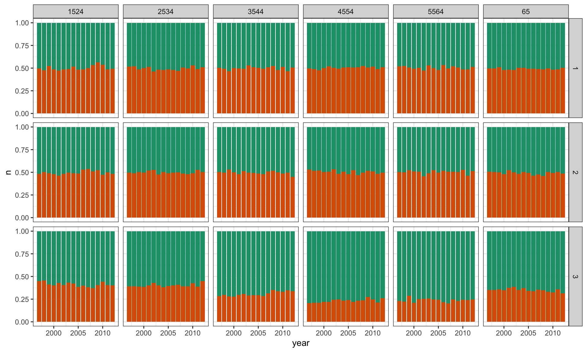

TB Lineup

A more complicated null

\(H_0\): Rates are the same across sex, regardless of age and year.
\(H_A\): They aren’t.

tbl <- tb_us |> group_by(sex) |> summarise(count=sum(count))
tbl
p <- tbl$count[1]/sum(tbl$count)

pos = sample(1:3, 1)
l <- lineup(null_dist(var="sex01", dist="binom",
                      list(size=1, p=p)),
            true=tb_us_long, n=3, pos=pos)
l <- l |>
  group_by(.sample, year, age) |>
  count(sex01)

1

Compute proportion across all data

2

Create lineup, with null data sampled from a Binomial() distribution with the sample proportion as \(p\)

3

Compute aggregate results

# A tibble: 2 × 2
  sex   count
  <chr> <dbl>
1 f     25915
2 m     55640

TB Lineup

ggplot(l, aes(x = year, y = n, fill = factor(sex01))) +
  geom_bar(stat = "identity", position = "fill") +
  facet_grid(.sample ~ age) +
  scale_fill_brewer(palette="Dark2") + 
  theme(legend.position="none")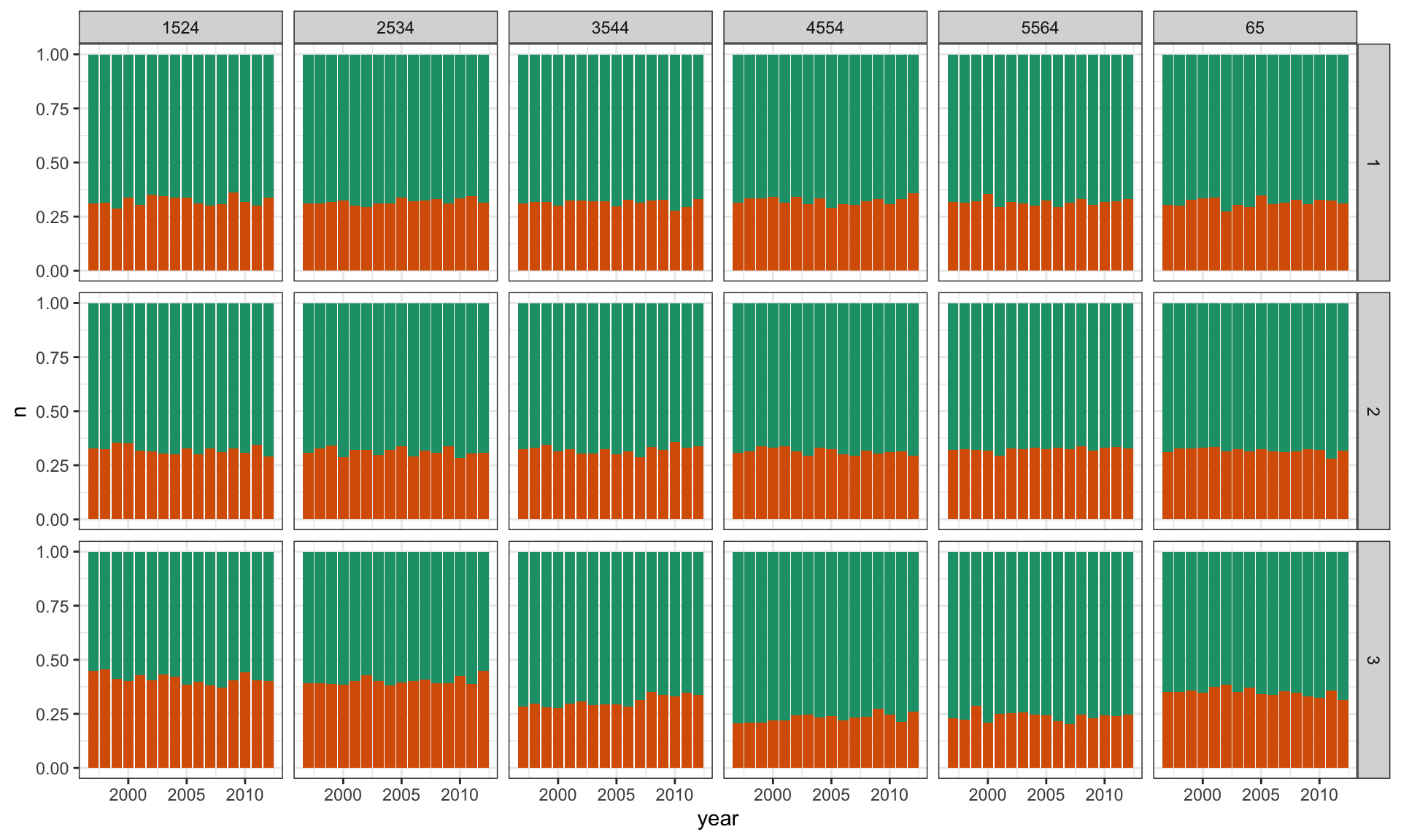

TB Lineup

Danger zone

• \(H_0\) is determined based on the plot type

• \(H_0\) is not based on the structure seen in the data set

• Null data creation method does not match characteristics of original sample other than that in \(H_0\)

A map lineup example

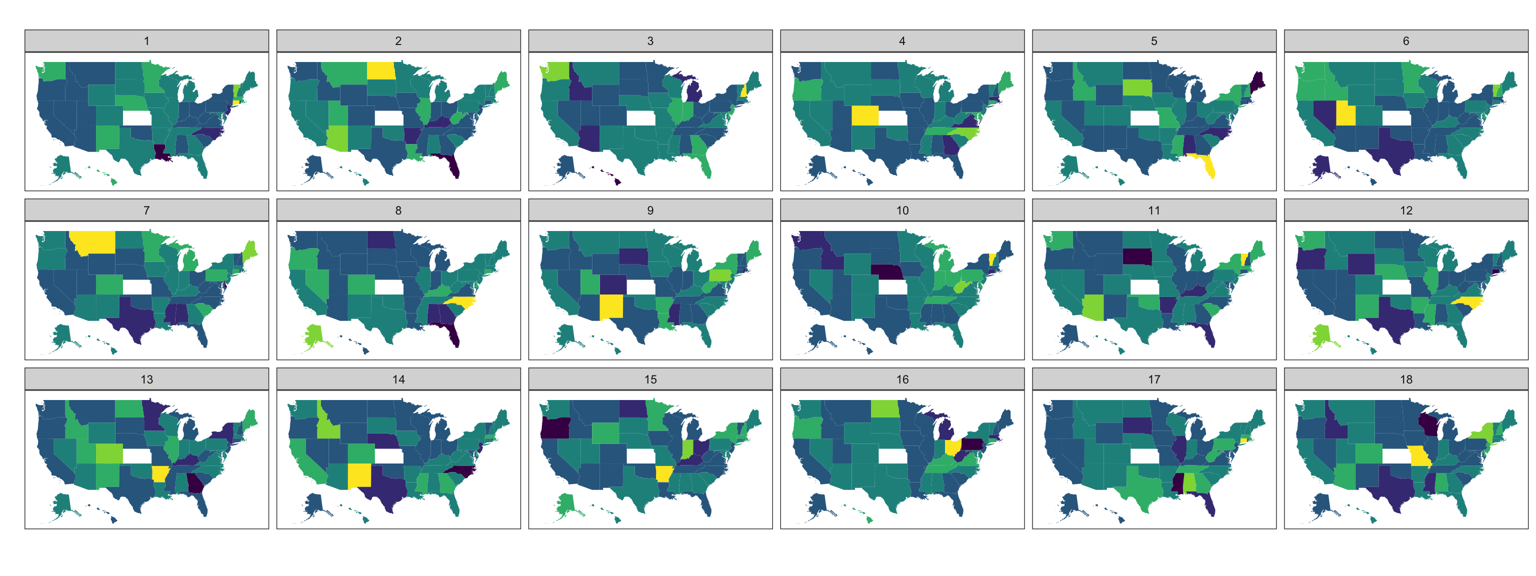
Does one map show a spatial trend?

Cancer incidence across the US 2010-2014, Melanoma cases per 100k. Data source: American Cancer Society.

Your turn

1. run this code,
2. look at your lineup (and only your lineup)
3. choose a plot
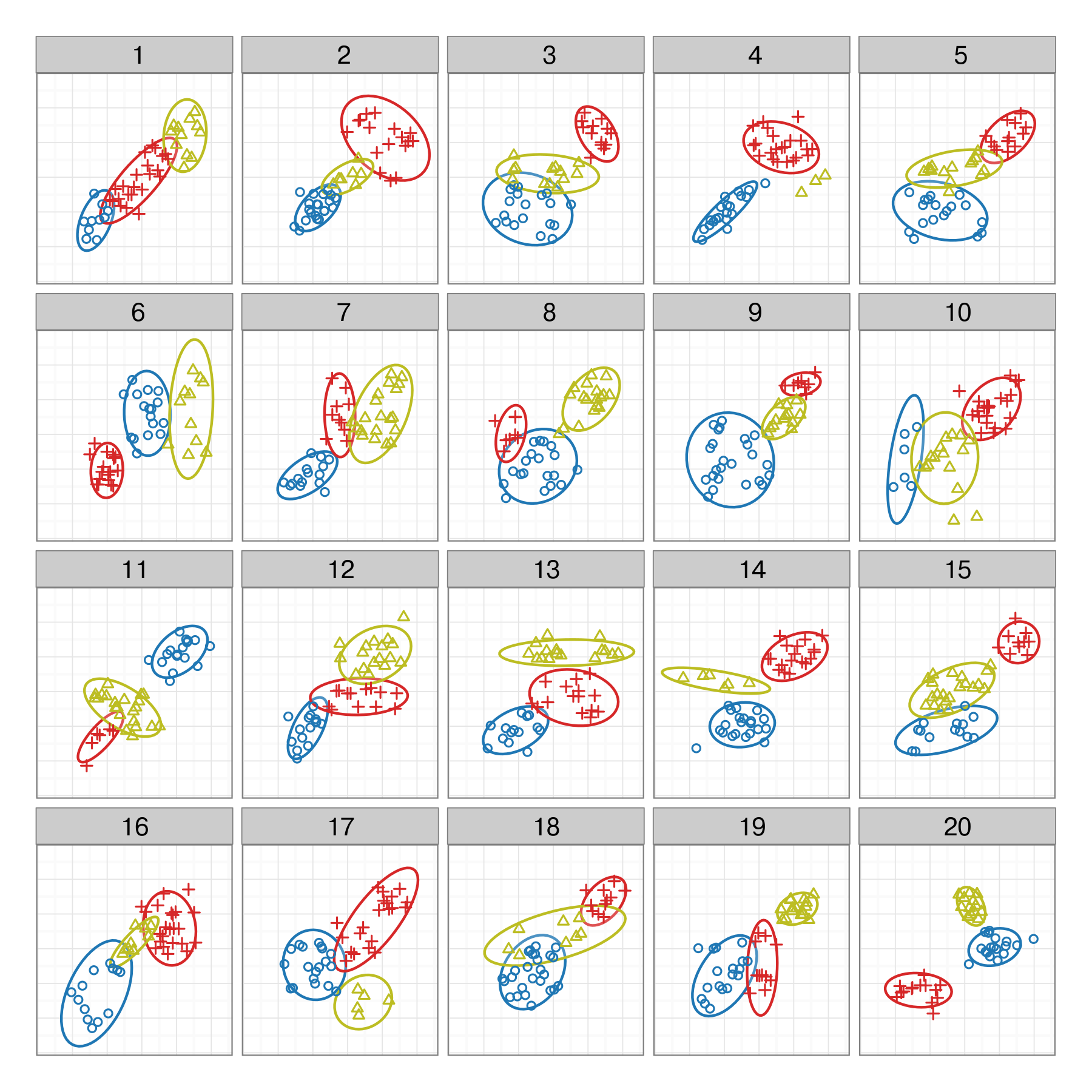
4. run the decrypt line
5. calculate x for your group
6. use the pvisual function to compute the p-value, K= group size, m=18
7. Try different \(\alpha\) values with pVis - how much difference does it make?

data(wasps)
lda_pred <- function(x) {
  d <- predict(lda(Group~., 
                   data=x[,-43]))$x[,1:2] |>
  as_tibble() |>
  mutate(Group = x$Group)
  return(d)
}
wasps_lineup <- lineup(null_permute('Group'), 
                       wasps[,-1], n=12) |>
  as_tibble()
wasps_lineup_lda <- wasps_lineup |>
  split(.$.sample) |>
  map_df(~lda_pred(.)) |>
  mutate(.sample = wasps_lineup$.sample)
ggplot(wasps_lineup_lda, aes(x=LD1, y=LD2, 
                             colour=Group)) + 
  geom_point() +
  facet_wrap(~.sample, ncol=4) +
  scale_colour_brewer(palette="Dark2") +
  theme(legend.position="none")

Enter the p-value in the chat!

Resources

• VanderPlas S., Röttger C., Cook D., Hofmann H.: Statistical Significance Calculations for Scenarios in Visual Inference, STAT, 2020, doi:http://dx.doi.org/10.1002/sta4.337.
• Hofmann, H., Follett, L., Majumder, M. and Cook, D. (2012) Graphical Tests for Power Comparison of Competing Designs, http://doi.ieeecomputersociety.org/10.1109/TVCG.2012.230.
• Wickham, H., Cook, D., Hofmann, H. and Buja, A. (2010) Graphical Inference for Infovis, http://doi.ieeecomputersociety.org/10.1109/TVCG.2010.161.
• Sievert, C. (2019) Interactive web-based data visualization with R, plotly, and shiny, https://plotly-r.com/index.html

This work is licensed under a Creative Commons Attribution-NonCommercial-ShareAlike 4.0 International License.