Tidying your data

SISBID 2025
https://github.com/dicook/SISBID

Using `tidyr`, `dplyr`

Writing readable code using pipes
What is tidy data? Why do you want tidy data? Getting your data into tidy form using tidyr.
Reading different data formats
String operations, working with text

The pipe operator `%>%` or `|>`

read as then
x %>% f(y) and x |> f(y) is the same as f(x, y)
%>% is part of the dplyr package (really, magrittr), |> is part of base R
pipes structure code as sequence of operations – as opposed to function order g(f(x))

The pipe operator `%>%` or `|>`

%>% is part of dplyr package (or more precisely, the magrittr package)
R 4.1 introduced the |> base pipe (no package necessary)
An explanation of the (subtle) differences between the pipes can be found here

tb <- read_csv(here::here("data/TB_notifications_2025-07-22.csv"))
tb   %>%                                # first we get the tb data
  filter(year == 2023) %>%              # then we focus on the most recent year
  group_by(country) %>%                 # then we group by country
  summarize(
    cases = sum(c_newinc, na.rm=TRUE)   # to create a summary of all new cases
    ) %>%
  arrange(desc(cases))                  # then we sort countries to show highest number of new cases first

tb <- read_csv(here::here("data/TB_notifications_2025-07-22.csv"))
tb |>                                  # first we get the tb data
  filter(year == 2023) |>              # then we focus on the most recent year
  group_by(country) |>                 # then we group by country
  summarize(
    cases = sum(c_newinc, na.rm=TRUE)   # to create a summary of all new cases
    ) |> 
  arrange(desc(cases))                  # then we sort countries to show highest number new cases first

# A tibble: 215 × 2
   country                            cases
   <chr>                              <dbl>
 1 India                            2382714
 2 Indonesia                         804836
 3 Philippines                       575770
 4 China                             564918
 5 Pakistan                          475761
 6 Nigeria                           367250
 7 Bangladesh                        302813
 8 Democratic Republic of the Congo  258069
 9 South Africa                      211810
10 Ethiopia                          134873
# ℹ 205 more rows

What is tidy data?

Illustrations from the Openscapes blog Tidy Data for reproducibility, efficiency, and collaboration by Julia Lowndes and Allison Horst

What do we expect tidy data to look like?
maybe easier: what are sources of messiness?

🔮 👽 👼 TWO MINUTE CHALLENGE

What are aspects of messiness in data that you have encountered?

Go to menti.com and enter code 2979 2396

Varying degree of messiness

Cryptic Names
More cryptic
Most
Too_much_info
Tables
Gross on repeat

What are the variables? Where are they located?

# A tibble: 6 × 4
  Inst                     AvNumPubs AvNumCits PctCompletion
  <chr>                        <dbl>     <dbl>         <dbl>
1 ARIZONA STATE UNIVERSITY      0.9       1.57          31.7
2 AUBURN UNIVERSITY             0.79      0.64          44.4
3 BOSTON COLLEGE                0.51      1.03          46.8
4 BOSTON UNIVERSITY             0.49      2.66          34.2
5 BRANDEIS UNIVERSITY           0.3       3.03          48.7
6 BROWN UNIVERSITY              0.84      2.31          54.6

What’s in the column names of this data? What are the experimental units? What are the measured variables?

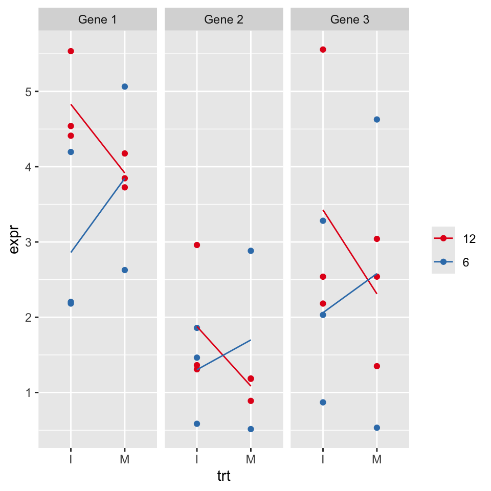
# A tibble: 3 × 12
  id     `WI-6.R1` `WI-6.R2` `WI-6.R4` `WM-6.R1` `WM-6.R2` `WI-12.R1` `WI-12.R2`
  <chr>      <dbl>     <dbl>     <dbl>     <dbl>     <dbl>      <dbl>      <dbl>
1 Gene 1      2.18     2.20       4.20     2.63       5.06       4.54       5.53
2 Gene 2      1.46     0.585      1.86     0.515      2.88       1.36       2.96
3 Gene 3      2.03     0.870      3.28     0.533      4.63       2.18       5.56
# ℹ 4 more variables: `WI-12.R4` <dbl>, `WM-12.R1` <dbl>, `WM-12.R2` <dbl>,
#   `WM-12.R4` <dbl>

What are the variables? What are the records?

           V1   V2 V3   V4  V5  V9 V13 V17 V21 V25 V29 V33 V37 V41 V45 V49 V53
1 ASN00086282 1970  7 TMAX 141 124 113 123 148 149 139 153 123 108 119 112 126
2 ASN00086282 1970  7 TMIN  80  63  36  57  69  47  84  78  49  42  48  56  51
3 ASN00086282 1970  7 PRCP   3  30   0   0  36   3   0   0  10  23   3   0   5
4 ASN00086282 1970  8 TMAX 145 128 150 122 109 112 116 142 166 127 117 127 159
5 ASN00086282 1970  8 TMIN  50  61  75  67  41  51  48  -7  56  62  47  33  67
6 ASN00086282 1970  8 PRCP   0  66   0  53  13   3   8   0   0   0   3   5   0
  V57 V61 V65 V69 V73 V77 V81 V85 V89 V93 V97
1 112 115 133 134 126 104 143 141 134 117 142
2  36  44  39  40  58  15  33  51  74  39  66
3   0   0   0   0   0   8   0  18   0   0   0
4 143 114  65 113 125 129 147 161 168 178 161
5  84  11  41  18  50  22  28  74  94  73  88
6   0  64   3  99  36   8   0   0   0   8  36

What are the variables? What are the experimental units?

# A tibble: 6 × 22
  iso2   year  m_04 m_514 m_014 m_1524 m_2534 m_3544 m_4554 m_5564  m_65   m_u
  <chr> <dbl> <dbl> <dbl> <dbl>  <dbl>  <dbl>  <dbl>  <dbl>  <dbl> <dbl> <dbl>
1 ZW     2003    NA    NA   133    874   3048   2228    981    367   205    NA
2 ZW     2004    NA    NA   187    833   2908   2298   1056    366   198    NA
3 ZW     2005    NA    NA   210    837   2264   1855    762    295   656    NA
4 ZW     2006    NA    NA   215    736   2391   1939    896    348   199    NA
5 ZW     2007     6   132   138    500   3693      0    716    292   153    NA
6 ZW     2008    NA    NA   127    614      0   3316    704    263   185     0
# ℹ 10 more variables: f_04 <dbl>, f_514 <dbl>, f_014 <dbl>, f_1524 <dbl>,
#   f_2534 <dbl>, f_3544 <dbl>, f_4554 <dbl>, f_5564 <dbl>, f_65 <dbl>,
#   f_u <dbl>

What are the variables? What are the observations?

            religion <$10k $10-20k $20-30k $30-40k
1           Agnostic    27      34      60      81
2            Atheist    12      27      37      52
3           Buddhist    27      21      30      34
4           Catholic   418     617     732     670
5 Don’t know/refused    15      14      15      11

10 week sensory experiment, 12 individuals assessed taste of french fries on several scales (how potato-y, buttery, grassy, rancid, paint-y do they taste?), fried in one of 3 different oils, replicated twice.

First few rows:

# A tibble: 4 × 9
  time  treatment subject   rep potato buttery grassy rancid painty
  <fct> <fct>     <fct>   <dbl>  <dbl>   <dbl>  <dbl>  <dbl>  <dbl>
1 1     1         3           1    2.9     0      0      0      5.5
2 1     1         3           2   14       0      0      1.1    0  
3 1     1         10          1   11       6.4    0      0      0  
4 1     1         10          2    9.9     5.9    2.9    2.2    0

What is the experimental unit? What are the factors of the experiment? What was measured? What do you want to know?

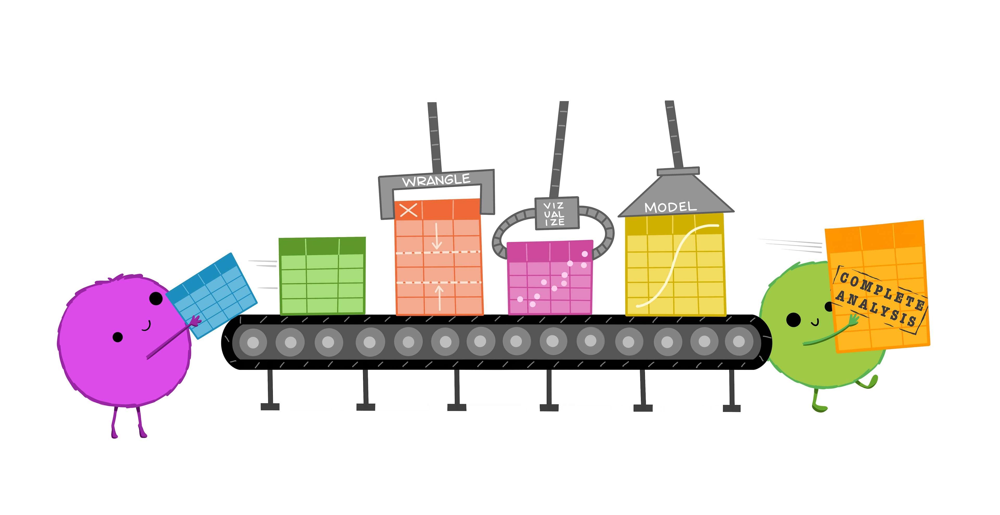
Messy data patterns

There are various features of messy data that one can observe in practice. Here are some of the more commonly observed patterns:

Column headers are not just variable names, but also contain values
Variables are stored in both rows and columns, contingency table format
One type of experimental unit stored in multiple tables
Dates in many different formats

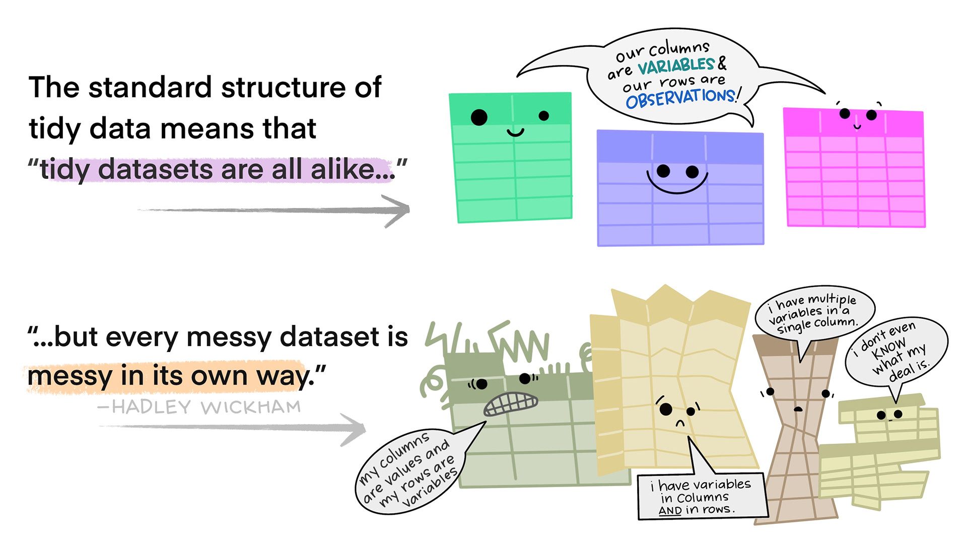
Tidy Data Conventions

Data is contained in a single table
Each observation forms a row (no data info in column names)
Each variable forms a column (no mashup of multiple pieces of information)

Long and Wide

Long form: one measured value per row. All other variables are descriptors (key variables) - good for modelling, terrible for most other analyses, e.g. correlation matrix
Widest form: all measured values for an entity are in a single row.
Wide form: measurements are arranged by some of the descriptors in columns (for direct comparisons)

Tidy verbs

pivot_longer: get information out of names into columns
pivot_wider: make columns of observed data for levels of design variables (for comparisons)
separate/unite: split and combine columns
nest/unnest: make/unmake variables into sub-data frames of a list variable

Pivot to long form

data |> pivot_longer(cols, names_to = "name", values_to = "value", ...)

pivot_longer turns a wide format into a long format
two new variables are introduced (in key-value format): name and value
col defines which variables should be combined

tidyr cheat sheet

Pivoting: an example

# wide format
dframe
  id trtA trtB
1  1  2.5   45
2  2  4.6   35

# long format
dframe |> pivot_longer(trtA:trtB, names_to="treatment", values_to="outcome")
# A tibble: 4 × 3
     id treatment outcome
  <int> <chr>       <dbl>
1     1 trtA          2.5
2     1 trtB         45  
3     2 trtA          4.6
4     2 trtB         35

Variable Selectors

data |> pivot_longer(cols, names_to = "key", values_to = "value", ...)
cols argument identifies variables that should be combined.
Pattern Selectors can be used to identify variables by name, position, a range (using :), a pattern, or a combination of all.

Examples of pattern selectors

starts_with(match, ignore.case = TRUE, vars = NULL)
other select functions: ends_with, contains, matches.
For more details, see ?tidyselect::language

TB notifications

New notifications of TB have the form new_sp_<sex><age group>:

read_csv(here::here("data/TB_notifications_2025-07-22.csv")) |> 
  dplyr::select(country, iso3, year, starts_with("new_sp_")) |>
  na.omit() |>
  head()
# A tibble: 6 × 23
  country     iso3   year new_sp_m04 new_sp_m514 new_sp_m014 new_sp_m1524
  <chr>       <chr> <dbl>      <dbl>       <dbl>       <dbl>        <dbl>
1 Afghanistan AFG    2010          4         193         197          986
2 Afghanistan AFG    2012          0         188         188         1116
3 Albania     ALB    2005          0           0           0           26
4 Albania     ALB    2006          1           4           5           24
5 Albania     ALB    2007          0           0           0           19
6 Albania     ALB    2009          0           0           0           22
# ℹ 16 more variables: new_sp_m2534 <dbl>, new_sp_m3544 <dbl>,
#   new_sp_m4554 <dbl>, new_sp_m5564 <dbl>, new_sp_m65 <dbl>, new_sp_mu <dbl>,
#   new_sp_f04 <dbl>, new_sp_f514 <dbl>, new_sp_f014 <dbl>, new_sp_f1524 <dbl>,
#   new_sp_f2534 <dbl>, new_sp_f3544 <dbl>, new_sp_f4554 <dbl>,
#   new_sp_f5564 <dbl>, new_sp_f65 <dbl>, new_sp_fu <dbl>

Pivot Longer: TB notifications

create two new variables: name and value

name contains all variable names starting with “new_sp_”
value contains all values of the selected variables

tb1 <- read_csv(here::here("data/TB_notifications_2025-07-22.csv")) |> 
  dplyr::select(country, iso3, year, starts_with("new_sp_")) |>
  pivot_longer(starts_with("new_sp_")) 

tb1 |> na.omit() |> head()
# A tibble: 6 × 5
  country     iso3   year name         value
  <chr>       <chr> <dbl> <chr>        <dbl>
1 Afghanistan AFG    1997 new_sp_m014      0
2 Afghanistan AFG    1997 new_sp_m1524    10
3 Afghanistan AFG    1997 new_sp_m2534     6
4 Afghanistan AFG    1997 new_sp_m3544     3
5 Afghanistan AFG    1997 new_sp_m4554     5
6 Afghanistan AFG    1997 new_sp_m5564     2

Separate columns

data |> separate_wider_delim (col, delim, names, ...)

split column col from data frame frame into a set of columns as specified in names
delim is the delimiter at which we split into columns, splitting separator.

Separate TB notifications

Work on name:

tb2 <- tb1 |>
  separate_wider_delim(
    name, delim = "_", 
    names=c("toss_new", "toss_sp", "sexage")) 

tb2 |> na.omit() |> head()
# A tibble: 6 × 7
  country     iso3   year toss_new toss_sp sexage value
  <chr>       <chr> <dbl> <chr>    <chr>   <chr>  <dbl>
1 Afghanistan AFG    1997 new      sp      m014       0
2 Afghanistan AFG    1997 new      sp      m1524     10
3 Afghanistan AFG    1997 new      sp      m2534      6
4 Afghanistan AFG    1997 new      sp      m3544      3
5 Afghanistan AFG    1997 new      sp      m4554      5
6 Afghanistan AFG    1997 new      sp      m5564      2

Separate columns

data %>% separate_wider_position(col, widths, ...)

split column col from frame into a set of columns specified in widths
widths is named numeric vector where the names become column names; unnamed components will be matched but not included.

Separate TB notifications again

Now split sexage into first character (m/f) and rest.

tb3 <- tb2 %>% dplyr::select(-starts_with("toss")) |> # remove the `toss` variables
  separate_wider_position(
    sexage,
    widths = c(sex = 1, age = 4),
    too_few = "align_start"
  )

tb3 |> na.omit() |> head()
# A tibble: 6 × 6
  country     iso3   year sex   age   value
  <chr>       <chr> <dbl> <chr> <chr> <dbl>
1 Afghanistan AFG    1997 m     014       0
2 Afghanistan AFG    1997 m     1524     10
3 Afghanistan AFG    1997 m     2534      6
4 Afghanistan AFG    1997 m     3544      3
5 Afghanistan AFG    1997 m     4554      5
6 Afghanistan AFG    1997 m     5564      2

Your turn

Read the genes data from folder data. Column names contain data and are kind of messy.

genes <- read_csv(here::here("data/genes.csv"))

names(genes)
 [1] "id"       "WI-6.R1"  "WI-6.R2"  "WI-6.R4"  "WM-6.R1"  "WM-6.R2" 
 [7] "WI-12.R1" "WI-12.R2" "WI-12.R4" "WM-12.R1" "WM-12.R2" "WM-12.R4"

Produce the data frame called gtidy as shown below:

head(gtidy)
# A tibble: 6 × 5
  id     trt   time  rep    expr
  <chr>  <chr> <chr> <chr> <dbl>
1 Gene 1 I     6     1      2.18
2 Gene 1 I     6     2      2.20
3 Gene 1 I     6     4      4.20
4 Gene 1 M     6     1      2.63
5 Gene 1 M     6     2      5.06
6 Gene 1 I     12    1      4.54

Plot the genes data overlaid with group means

gmean <- gtidy |> 
  group_by(id, trt, time) |> 
  summarise(expr = mean(expr))
gtidy |> 
  ggplot(aes(x = trt, y = expr, colour=time)) +
  geom_point() +
  geom_line(data = gmean, aes(group = time)) +
  facet_wrap(~id) +
  scale_colour_brewer("", palette="Set1")

Resources

This work is licensed under a Creative Commons Attribution-NonCommercial-ShareAlike 4.0 International License.

Tidying your data

Using tidyr, dplyr

The pipe operator %>% or |>

The pipe operator %>% or |>

Pipe Example

What is tidy data?

🔮 👽 👼 TWO MINUTE CHALLENGE

Varying degree of messiness

Messy data patterns

Tidy Data Conventions

Long and Wide

Tidy verbs

Pivot to long form

Pivoting: an example

Variable Selectors

Examples of pattern selectors

TB notifications

Pivot Longer: TB notifications

Separate columns

Separate TB notifications

Separate columns

Separate TB notifications again

Your turn

Plot the genes data overlaid with group means

Resources

Using `tidyr`, `dplyr`

The pipe operator `%>%` or `|>`

The pipe operator `%>%` or `|>`