Load libraries
source("code/setup.R")The tree algorithm (Breiman et al., 1984) is a simple and versatile algorithmic method for supervised classification. The basic tree algorithm generates a classification rule by sequentially splitting the data into two buckets. Splits are made between sorted data values of individual variables, with the goal of obtaining pure classes on each side of the split. The inputs for a simple tree classifier commonly include (1) an impurity measure, an indication of the relative diversity among the cases in the terminal nodes; (2) a parameter that sets the minimum number of cases in a node, or the minimum number of observations in a terminal node of the tree; and (3) a complexity measure that controls the growth of a tree, balancing the use of a simple generalizable tree against a more accurate tree tailored to the sample. When applying tree methods, exploring the effects of the input parameters on the tree is instructive; for example, it helps us to assess the stability of the tree model.
Although algorithmic models do not depend on distributional assumptions, that does not mean that every algorithm is suitable for all data. For example, the tree model works best when all variables are independent within each class, because it does not take such dependencies into account. Visualization can help us to determine whether a particular model should be applied. In classification problems, it is useful to explore the cluster structure, comparing the clusters with the classes and looking for evidence of correlation within each class. The plots in Figure 14.2 and Figure 14.4 shows a strong correlation between the variables within each species, which indicates that the tree model may not give good results for the penguins data. We’ll show how this is the case with two variables initially, and then extend to the four variables.
source("code/setup.R")load("data/penguins_sub.rda")
p_bl_bd_tree <- rpart(species~bl+bd, data=penguins_sub)
#f1 <- rpart.plot(p_bl_bd_tree, box.palette="Grays")
d <- dendro_data(p_bl_bd_tree)
f1 <- ggplot() +
geom_segment(data = d$segments,
aes(x = x, y = y,
xend = xend, yend = yend)) +
geom_text(data = d$labels,
aes(x = x, y = y,
label = label), size = 2.7,
vjust = 1.2) +
geom_text(data = d$leaf_labels,
aes(x = x, y = y,
label = label), size = 2.5,
vjust = 2, hjust=c(0,0.5,0,0.5)) +
expand_limits(x=0.9, y=0) +
theme_dendro()
p_bl_bd_tree_boundaries <- explore(p_bl_bd_tree, penguins_sub)
f2 <- ggplot(p_bl_bd_tree_boundaries) +
geom_point(aes(x=bl, y=bd, colour=species, shape=.TYPE)) +
scale_color_discrete_divergingx(palette="Zissou 1") +
scale_shape_manual(values=c(46, 16)) +
theme_minimal() +
theme(aspect.ratio = 1, legend.position = "none")
f1 + f2 + plot_layout(ncol=2)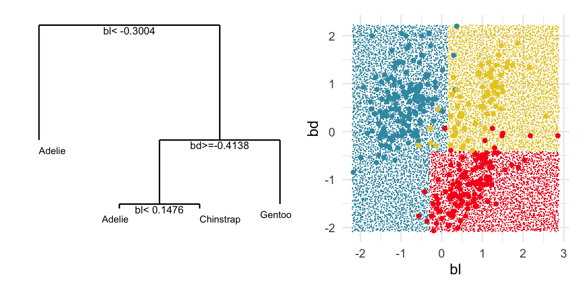
The plots in Figure 15.1 show the inadequacies of the tree fit. The background color indicates the class predictions, and thus boundaries produced by the tree fit. They can be seen to be boxy, and missing the elliptical nature of the penguin clusters. This produces errors in the classification of observations which are indefensible. One could always force the tree to fit the data more closely by adjusting the parameters, but the main problem persists: that one is trying to fit elliptical shapes using boxes.
There are less strict assumptions for a non-parametric model but it is still important to understand the model fit relative to the data.
The boundaries for the tree model on all four variables of the penguins data can be viewed similarly, by predicting a set of points randomly generated in the 4D domain of observed values. Figure 15.2 shows the prediction regions for LDA and a default tree in a slice tour (Laa et al., 2020). The slice tour is used to help see into the middle of the 4D cube. It slices the cube through the centre of the data, where the boundaries of the regions should meet.
The prediction regions of the default fitted tree are shown in comparison to those from the LDA model. We don’t show the tree diagram here, but it makes only six splits of the tree model, which is delightfully simple. However, just like the model fitted to two variables, the result is not adequate for the penguins data. The tree model generates boxy boundaries, whereas the LDA model splits the 4D cube obliquely. The boxy regions don’t capture the differences between the elliptically-shaped clusters. Overlaying the observed data on this display would make this clearer, but the boundaries are easier to examine without them.
p_tree <- rpart(species~., data=penguins_sub[,1:5])
rpart.plot(p_tree, box.palette="Grays")

p_tree_boundaries <- explore(p_tree, penguins_sub)
animate_slice(p_tree_boundaries[p_tree_boundaries$.TYPE == "simulated",1:4], col=p_tree_boundaries[p_tree_boundaries$.TYPE == "simulated",6], v_rel=0.02, axes="bottomleft")
load("data/penguins_tour_path.rda")
render_gif(p_tree_boundaries[p_tree_boundaries$.TYPE == "simulated",1:4],
           planned_tour(pt1),
           display_slice(v_rel=0.02,
             col=p_tree_boundaries[p_tree_boundaries$.TYPE == "simulated",6],
             axes="bottomleft"),                     gif_file="gifs/penguins_tree_boundaries.gif",
           frames=500,
           loop=FALSE
           )
With the penguins data, a tree model may not be a good choice due to the strong correlation between variables. The best separation is in combinations of variables, not the single variable tree splits.
A random forest (Breiman, 2001) is a classifier that is built from multiple trees generated by randomly sampling the cases and the variables. The random sampling (with replacement) of cases has the fortunate effect of creating a training (“in-bag”) and a test (“out-of-bag”) sample for each tree computed. The class of each case in the out-of-bag sample for each tree is predicted, and the predictions for all trees are combined into a vote for the class identity.
A random forest is a computationally intensive method, a “black box” classifier, but it produces several diagnostics that make the outcome less mysterious. Some diagnostics that help us to assess the model are the votes, the measure of variable importance, and the proximity matrix.
Here we show how to use the randomForest (Liaw & Wiener, 2002) votes matrix for the penguins data to investigate confusion between classes, and observations which are problematic to classify. The votes matrix can be considered to be a predictive probability distribution, where the values for each observation sum to 1. With only three classes the votes matrix is only a 2D object, and thus easy to examine. With four or more classes the votes matrix needs to be examined in a tour.
penguins_rf <- randomForest(species~.,
                             data=penguins_sub[,1:5],
importance=TRUE)penguins_rf
Call:
 randomForest(formula = species ~ ., data = penguins_sub[, 1:5],      importance = TRUE)
               Type of random forest: classification
                     Number of trees: 500
No. of variables tried at each split: 2

        OOB estimate of  error rate: 2.4%
Confusion matrix:
          Adelie Chinstrap Gentoo class.error
Adelie       143         3      0 0.020547945
Chinstrap      4        64      0 0.058823529
Gentoo         0         1    118 0.008403361
To examine the votes matrix, we extract the votes element from the random forest model object. The first five rows are:
head(penguins_rf$votes, 5) Adelie Chinstrap Gentoo
1 1.0000 0.000000 0
2 0.9703 0.029703 0
3 0.9951 0.004926 0
4 1.0000 0.000000 0
5 1.0000 0.000000 0This has three columns corresponding to the three species, but because each row is a set of proportions it is only a 2D object. To reduce the dimension from 3D to the 2D we use a Helmert matrix (Lancaster, 1965). A Helmert matrix has a first row of all 1’s. The remaining components of the matrix are 1’s in the lower triangle, and 0’s in the upper triangle and the diagonal elements are the negative row sum. The rows are usually normalised to have length 1. They are used to create contrasts to test combinations of factor levels for post-testing after Analysis of Variance (ANOVA). For compositional data, like the votes matrix, when the first row is removed a Helmert matrix can be used to reduce the dimension appropriately. For three classes, this will generate the common 2D ternary diagram, but for higher dimensions it will reduce to a \((g-1)\)-dimensional simplex. For the penguins data, the Helmert matrix for 3D is
geozoo::f_helmert(3) [,1] [,2] [,3]
helmert 0.5774 0.5774 0.5774
x 0.7071 -0.7071 0.0000
x 0.4082 0.4082 -0.8165We drop the first row, transpose it, and use matrix multiplication with the votes matrix to get the ternary diagram.
# Add simplex
simp <- simplex(p=2)
sp <- data.frame(cbind(simp$points), simp$points[c(2,3,1),])
colnames(sp) <- c("x1", "x2", "x3", "x4")
sp$species = sort(unique(penguins_sub$species))
p_ternary <- ggplot() +
  geom_segment(data=sp, aes(x=x1, y=x2, xend=x3, yend=x4)) +
  geom_text(data=sp, aes(x=x1, y=x2, label=species),
            nudge_x=c(-0.06, 0.07, 0),
            nudge_y=c(0.05, 0.05, -0.05)) +
  geom_point(data=p_rf_v_p, aes(x=x1, y=x2,
                                colour=species),
             size=2, alpha=0.5) +
  scale_color_discrete_divergingx(palette="Zissou 1") +
  theme_map() +
theme(aspect.ratio=1, legend.position="none")# Look at the votes matrix, in its 3D space
animate_xy(penguins_rf$votes, col=penguins_sub$species)
# Save an animated gif
render_gif(penguins_rf$votes,
grand_tour(),
display_xy(v_rel=0.02,
col=penguins_sub$species,
axes="bottomleft"),
gif_file="gifs/penguins_rf_votes.gif",
frames=500,
loop=FALSE
)
We can use the geozoo package to generate the surrounding simplex, which for 2D is a triangle.
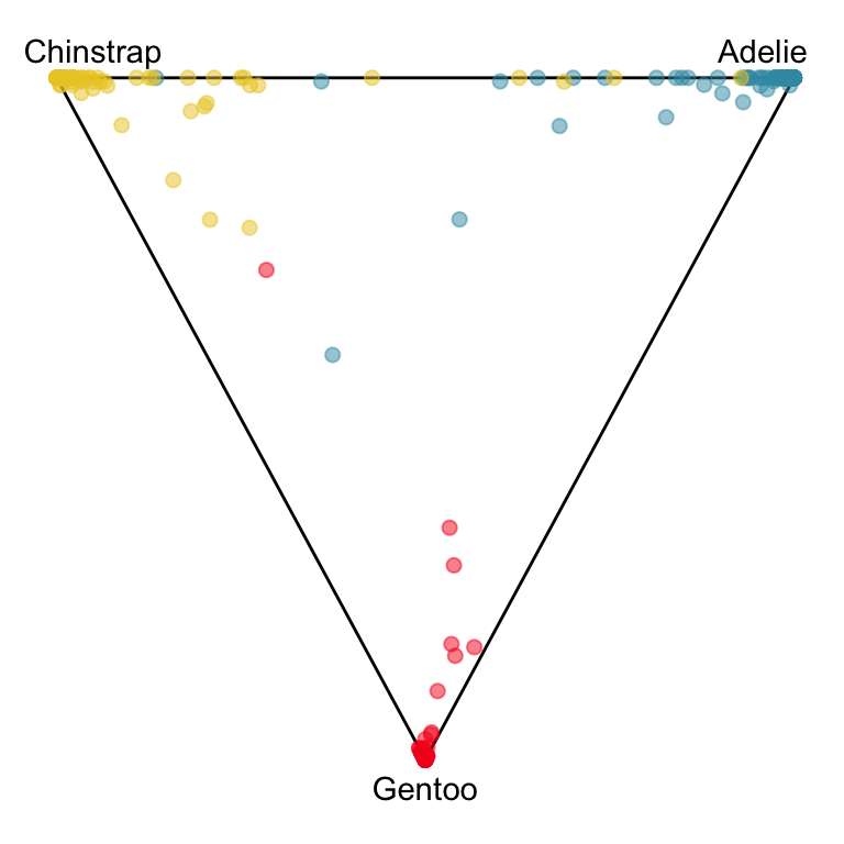
The votes matrix reports the proportion of trees each observation is classified as each class. From the tour of the votes matrix, as in Figure 15.3(a), it can be seen to be 2D in 3D space. This is due to the constraint that the three proportions for each observation sum to 1. Using a Helmert matrix, this data can be projected into the 2D space, or more generally the \((g-1)\)-dimensional space where it resides, shown in Figure 15.3(b). In 2D this is called a ternary diagram, and in higher dimensions the bounding shapes might be considered to be a simplex. The vertices of this shape correspond to \((1,0,0), (0,1,0), (0,0,1)\) (and analogously for higher dimensions), which represent perfect confidence, that an observation is classified into that group all the time.
What we can see here is a concentration of points in the corners of the triangle, this indicates that most of the penguins are confidently classified into their correct class. Then there is more separation between the Gentoo and the others, than between Chinstrap and Adelie. That means that as a group Gentoo are more distinguishable. Only one of the Gentoo penguins has substantial confusion, mostly confused as a Chinstrap, but occasionally confused as an Adelie – if it was only ever confused as a Chinstrap it would fall on the edge between Gentoo and Chinstrap. There are quite a few Chinstrap and Adelie penguins confused as each other, with a couple of each more confidently predicted to be the other class. This can be seen because there are points of the wrong colour close to those vertices.
The votes matrix is useful for investigating the fit, but one should remember that there are some structural elements of the penguins data that don’t lend themselves to tree models. Although a forest has the capacity to generate non-linear boundaries by combining predictions from multiple trees, it is still based on the boxy boundaries of trees. This makes it less suitable for the penguins data with elliptical classes. You could use the techniques from the previous section to explore the boundaries produced by the forest, and you will find that the are more boxy than the LDA models.
By visualising the votes matrix we can understand which observations are harder to classify, which of the classes are more easily confused with each other.
To examine a vote matrix for a problem with more classes, we will examine the 10 class fake_trees data example. The full data has 100 variables, and we have seen from Chapter 7 that reducing to 10 principal components allows the linear branching structure in the data to be seen. Given that the branches correspond to the classes, it will be interesting to see how well the random forest model performs.
ft_pca <- prcomp(fake_trees[,1:100],
                 scale=TRUE, retx=TRUE)
ft_pc <- as.data.frame(ft_pca$x[,1:10])
ft_pc$branches <- fake_trees$branches

ft_rf <- randomForest(branches~., data=ft_pc,
importance=TRUE)head(ft_rf$votes, 5) 0 1 2 3 4 5 6 7 8 9
1 0.9 0 0.005 0.000 0.000 0.08 0 0 0.005 0.00
2 0.6 0 0.016 0.000 0.027 0.34 0 0 0.000 0.00
3 0.8 0 0.057 0.005 0.151 0.02 0 0 0.000 0.02
4 0.9 0 0.011 0.000 0.005 0.09 0 0 0.000 0.00
5 0.7 0 0.030 0.024 0.012 0.25 0 0 0.012 0.00ft_rf_votes <- ft_rf$votes |>
as_tibble() |>
mutate(branches = fake_trees$branches)
proj <- t(geozoo::f_helmert(10)[-1,])
f_rf_v_p <- as.matrix(ft_rf_votes[,1:10]) %*% proj
colnames(f_rf_v_p) <- c("x1", "x2", "x3", "x4", "x5", "x6", "x7", "x8", "x9")
f_rf_v_p <- f_rf_v_p |>
as.data.frame() |>
mutate(branches = fake_trees$branches)
simp <- geozoo::simplex(p=9)
sp <- data.frame(simp$points)
colnames(sp) <- c("x1", "x2", "x3", "x4", "x5", "x6", "x7", "x8", "x9")
sp$branches = ""
f_rf_v_p_s <- bind_rows(sp, f_rf_v_p) |>
mutate(branches = factor(branches))
labels <- c("0" , "1", "2", "3", "4", "5", "6", "7", "8", "9",
rep("", 3000))animate_xy(f_rf_v_p_s[,1:9], col = f_rf_v_p_s$branches,
axes = "off", half_range = 0.8,
edges = as.matrix(simp$edges),
obs_labels = labels, palette = "Viridis")
render_gif(f_rf_v_p_s[,1:9],
grand_tour(),
display_xy(col = f_rf_v_p_s$branches,
axes = "off", half_range = 0.8,
edges = as.matrix(simp$edges),
obs_labels = labels, palette="Viridis"),
gif_file="gifs/ft_votes.gif",
frames=500) 
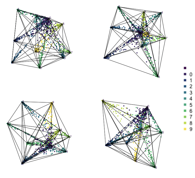
The votes matrix is 9D, due to the 9 groups. With this many dimensions, if the cluster structure is weak, it will look messy in a tour. However, what we can see in Figure 15.4 is that the structure is relatively simple, and very interesting in that it suggests a strong clustering of classes. Points are coloured by their true class. The lines represent the 8D simplex that bounds the observations, akin to the triangle in the ternary diagram.
Points concentrate at the vertices, which means that most are confidently predicted to be their true class. The most spread of points is along single edges, between pairs of vertices. This means that when there is confusion it is mostly with just one other group. One vertex (0) has connections to all other vertices. That is, there are points stretching from this vertex to every other. It means that some observations in every other class can be confused with class 0, and class 0 observations can be confused with every other class. This information suggests that cluster 0 is central to all the other clusters.
Some of this information could also be inferred from the confusion matrix for the model. However visualising the votes matrix provides more intricate details. Here we have seen that the points spread out from a vertex, with fewer and fewer the further one gets. It allows us to see the distribution of points, which is not possible from the confusion matrix alone. The same misclassification rate could be due to a variety of distributions. The visual pattern in the votes matrix is striking, and gives additional information about how the clustering distribution, and shapes of clusters, matches the class labels. It reinforces the clusters are linear extending into different dimensions in the 100D space, but really only into about 8D (as we’ll see from the variable importance explanation below). We also see that nine of the clusters are all connected to a single cluster.
The votes matrix for the fake trees has a striking geometric structure, with one central cluster connected to all other clusters, each of which is distinct from each other.
The variable importance score across all classes, and for each class is useful for choosing variables to enter into a tour, to explore class differences. This is particularly so when there are many variables, as in the fake_trees data. We would also expect that this data will have a difference between importance for some classes.
ft_rf$importance |>
  as_tibble(rownames="Var") |>
  rename(Acc=MeanDecreaseAccuracy,
         Gini=MeanDecreaseGini) |>
  #arrange(desc(Gini)) |>
  gt() |>
  fmt_number(columns = c(`0`,`1`,`2`,`3`,`4`,
                         `5`,`6`,`7`,`8`,`9`),
             decimals = 1) |>
  fmt_number(columns = Acc,
             decimals = 2) |>
  fmt_number(columns = Gini,
decimals = 0)| Var | 0 | 1 | 2 | 3 | 4 | 5 | 6 | 7 | 8 | 9 | Acc | Gini |
|---|---|---|---|---|---|---|---|---|---|---|---|---|
| PC1 | 0.1 | 0.4 | 0.4 | 0.3 | 0.2 | 0.5 | 0.4 | 0.2 | 0.3 | 0.3 | 0.31 | 484 |
| PC2 | 0.1 | 0.2 | 0.2 | 0.5 | 0.3 | 0.3 | 0.2 | 0.4 | 0.2 | 0.3 | 0.28 | 377 |
| PC3 | 0.1 | 0.1 | 0.1 | 0.1 | 0.5 | 0.1 | 0.1 | 0.1 | 0.2 | 0.2 | 0.16 | 302 |
| PC4 | 0.1 | 0.4 | 0.0 | 0.0 | 0.1 | 0.0 | 0.4 | 0.1 | 0.1 | 0.1 | 0.14 | 335 |
| PC5 | 0.1 | 0.1 | 0.3 | 0.1 | 0.2 | 0.2 | 0.1 | 0.1 | 0.3 | 0.2 | 0.18 | 337 |
| PC6 | 0.1 | 0.2 | 0.3 | 0.2 | 0.1 | 0.1 | 0.0 | 0.3 | 0.2 | 0.2 | 0.16 | 292 |
| PC7 | 0.1 | 0.0 | 0.2 | 0.0 | 0.1 | 0.1 | 0.1 | 0.3 | 0.1 | 0.1 | 0.11 | 249 |
| PC8 | 0.0 | 0.1 | 0.0 | 0.2 | 0.1 | 0.1 | 0.0 | 0.0 | 0.1 | 0.3 | 0.09 | 221 |
| PC9 | 0.1 | 0.0 | 0.0 | 0.0 | 0.0 | 0.0 | 0.0 | 0.0 | 0.1 | 0.0 | 0.02 | 58 |
| PC10 | 0.0 | 0.0 | 0.0 | 0.0 | 0.0 | 0.0 | 0.0 | 0.0 | 0.0 | 0.0 | 0.01 | 45 |
From the variable importance (Table 15.1), we can see that PC9 and PC10 do not substantially contribute. That means the 100D data can be reduced to 8D without losing the information about the cluster structure. PC1 is most important overall, and the order matches the PC order, as might be expected because highest variance corresponds to the most spread clusters. Each cluster has a different set of variables that are important. For example, the variables important for distinguishing cluster 1 are PC1 and PC4, and for cluster 2 they are PC1 and PC5.
Class-wise variable importance helps to find a subspace on which to tour to examine how this class cluster differs from the others.
We can use the accuracy information to choose variables to provide to the tour. Overall, one would sequentially add the variables into a tour based on their accuracy or Gini value. Here it is simply starting with the first three PCs, and then sequentially adding the PCs to examine how distinct the clusters are with and without the extra variable. It can be helpful to focus on a single class against all the others. To do this create a new binary class variable, indicating that the observation belongs to class \(k\) or not, as follows:
ft_pc <- ft_pc |>
  mutate(cl1 = factor(case_when(
                 branches == "0" ~ "0",
                 branches == "1" ~ "1",
                 .default = "other"
)))ft_pc_cl1 <- ggplot(ft_pc, aes(x=PC4, y=PC1, col=cl1)) +
geom_point(alpha=0.7, size=1) +
scale_color_discrete_sequential(palette="Viridis", rev=FALSE) +
theme_minimal() +
theme(aspect.ratio = 1)From Figure 15.5 we can see how cluster 1 is distinct from all of the other observations, albeit with a close connection to the trunk of the tree (cluster 0). The distinction is visible whenever PC4 contributes to the projection, but can be seen clearly with only PC1 and PC4.
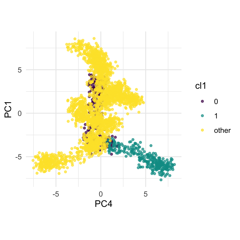
fake_trees data. The most important variables were PC1 and PC4. A combination of PC2 and PC4 reveals the difference between cluster 1 and all the other clusters.
For a problem like this, it can be useful to look at several classes together. We’ve chosen to start with class 8 (light green), because from Figure 15.4 it appears to have less connection with class 0, and closer connection with another class. This is class 6 (medium green) which also has one observation confused with class 8 according to the confusion matrix (printed below).
When we examine these two clusters in association with class 0, we can see that there is a third cluster that is connected with clusters 6 and 8. It turns out to be cluster 1. It’s confusing, because the confusion matrix would suggest that the overlap from all is with cluster 0, but not each other.
ft_rf$confusion 0 1 2 3 4 5 6 7 8 9 class.error
0 267 5 2 2 3 4 6 3 5 3 0.110
1 13 287 0 0 0 0 0 0 0 0 0.043
2 9 0 289 0 2 0 0 0 0 0 0.037
3 7 0 0 289 0 0 0 4 0 0 0.037
4 11 0 0 0 289 0 0 0 0 0 0.037
5 12 0 0 0 0 288 0 0 0 0 0.040
6 13 0 0 0 0 0 286 0 1 0 0.047
7 6 0 0 4 0 0 0 290 0 0 0.033
8 9 0 0 0 0 0 0 0 291 0 0.030
9 5 0 0 0 0 0 0 1 0 294 0.020ft_pc <- ft_pc |>
mutate(cl8 = factor(case_when(
branches == "0" ~ "0",
branches == "6" ~ "6",
branches == "1" ~ "1",
branches == "8" ~ "8",
.default = "other"
)))ft_pc_cl8 <- ggplot(ft_pc, aes(x=PC1, y=PC5, col=cl8)) +
geom_point(alpha=0.7, size=1) +
scale_color_discrete_sequential(palette="Viridis", rev=FALSE) +
theme_minimal() +
theme(aspect.ratio = 1)From the tour in Figure 15.6 we can see that clusters 1, 6, and 8 share one end of the trunk (cluster 0). Cluster 8 is almost more closely connected with cluster 6, though, than cluster 0. PC1 and PC5 mostly show the distinction between cluster 8 and the rest of the points, but it is clearer if more variables are used.
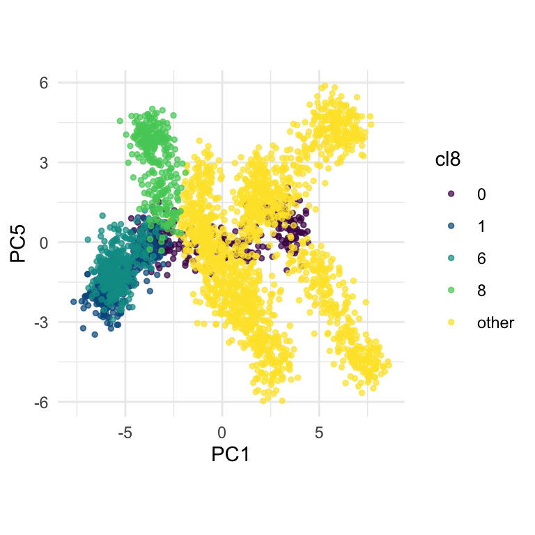
fake_trees data, relative to nearby clusters 1 and 6. The most important variables for cluster 8 are PC1, PC2, PC5, but to explore in association with clusters 1 and 6, we include PC4 and PC6. A combination of PC1 and PC5 reveals the difference between cluster 8, 6, 1 and 0.
Although the confusion matrix suggests that class clusters are separated except for class 0, focusing on a few classes and using the variable importance to examine smaller subspaces, reveals they are connected in groups of three to class 0.
Using a grand tour compare the boundaries from the random forest model on the penguins data to that of (a) a default tree model, (b) an LDA model. Is it less boxy than the tree model, but still more boxy than that of the LDA model?
Tinker with the parameters of the tree model to force it to fit a tree more closely to the data. Compare the boundaries from this with the default tree, and with the forest model. Is it less boxy than the default tree, but more boxy than the forest model?
Fit a random forest model to the bushfires data using the cause variable as the class. It is a highly imbalanced classification problem. What is the out-of-bag error rate for the forest? Are there some classes that have lower error rate than others? Examine the 4D votes matrix with a tour, and describe the confusion between classes. This is interesting because it is difficult to accurately classify the fire ignition cause, and only some groups are often confused with each other. You should be able to see this from the votes matrix.
Use this code to restrict the variables used in the model, appropriately:
Fit a forest model to the first 21 PCs of the sketches data. Explore the 5D votes matrix. Why does it look star-shaped?
Choose a cluster (or group of clusters) from the fake_trees data (2, 3, 4, 5, 7, 9) to explore in detail like done in Section 15.2.2. Be sure to choose which PCs are the most useful using a tour, and follow-up by making a scatterplot showing the best distinction between your chosen cluster and the other observations.
Using the aflw data (using the same subset of variables and players as used in Q3 of Chapter 13) compute:
position is removed for the calculation.)position.Discuss what is learned from each representation of the data, relative to the differences between skills of the players.
You can use this code to subset the data:
There are several interesting data sets with class variables available on the GGobi website. Examine the differences between type of music, based on the the variables lvar, lave, lmax, lfener, lfreq. Fit a random forest model using type as the variable. (It is best to remove the “New wave” class because there are too few observations.) Using the variable importance values, make plots of the top two variables, and then tour on the top three variables. Is two or three variables suffficient to distinguish between classical and rock music types?
The music data can be read using: