Wrangling Data and Models

SISBID 2026
https://github.com/dicook/SISBID

Outline

dplyr: motivation, functions, chaining
broom, broom.mixed: tidily extract elements from model summaries

# format the data
ff_long <- french_fries |> pivot_longer(potato:painty, names_to = "type", values_to = "rating")

dplyr verbs

There are five primary dplyr verbs, representing distinct data analysis tasks:

filter: Extract specified rows of a data frame
arrange: Reorder the rows of a data frame
select: Select specified columns of a data frame
mutate: Add new or transform a column of a data frame
summarise: Create collapsed summaries of a data frame
(group_by: Introduce structure to a data frame)

Filter

select a subset of the observations (horizontal selection)

load(here::here("data/french_fries.rda"))
french_fries |>
    filter(subject == 3, time == 1) #<<
# A tibble: 6 × 9
  time  treatment subject   rep potato buttery grassy rancid painty
* <fct> <fct>     <fct>   <dbl>  <dbl>   <dbl>  <dbl>  <dbl>  <dbl>
1 1     1         3           1    2.9     0      0      0      5.5
2 1     1         3           2   14       0      0      1.1    0  
3 1     2         3           1   13.9     0      0      3.9    0  
4 1     2         3           2   13.4     0.1    0      1.5    0  
5 1     3         3           1   14.1     0      0      1.1    0  
6 1     3         3           2    9.5     0      0.6    2.8    0

Arrange

order the observations (hierarchically)

french_fries |>
    arrange(desc(rancid)) |> #<<
    head()
# A tibble: 6 × 9
  time  treatment subject   rep potato buttery grassy rancid painty
  <fct> <fct>     <fct>   <dbl>  <dbl>   <dbl>  <dbl>  <dbl>  <dbl>
1 9     2         51          1    7.3     2.3      0   14.9    0.1
2 10    1         86          2    0.7     0        0   14.3   13.1
3 5     2         63          1    4.4     0        0   13.8    0.6
4 9     2         63          1    1.8     0        0   13.7   12.3
5 5     2         19          2    5.5     4.7      0   13.4    4.6
6 4     3         63          1    5.6     0        0   13.3    4.4

Select

select a subset of the variables (vertical selection)

french_fries |>
    select(time, treatment, subject, rep, potato) |> #<<
    head()
# A tibble: 6 × 5
  time  treatment subject   rep potato
  <fct> <fct>     <fct>   <dbl>  <dbl>
1 1     1         3           1    2.9
2 1     1         3           2   14  
3 1     1         10          1   11  
4 1     1         10          2    9.9
5 1     1         15          1    1.2
6 1     1         15          2    8.8

Summarise

summarize observations into a (set of) one-number statistic(s):

french_fries |>
    summarise( #<<
      mean_rancid = mean(rancid, na.rm=TRUE), 
      sd_rancid = sd(rancid, na.rm = TRUE)
      ) #<<
# A tibble: 1 × 2
  mean_rancid sd_rancid
        <dbl>     <dbl>
1        3.85      3.78

Summarise and group_by

french_fries |>
    group_by(time, treatment) |>
    summarise(mean_rancid = mean(rancid), sd_rancid = sd(rancid))
# A tibble: 30 × 4
# Groups:   time [10]
   time  treatment mean_rancid sd_rancid
   <fct> <fct>           <dbl>     <dbl>
 1 1     1                2.76      3.21
 2 1     2                1.72      2.71
 3 1     3                2.6       3.20
 4 2     1                3.9       4.37
 5 2     2                2.14      3.12
 6 2     3                2.50      3.38
 7 3     1                4.65      3.93
 8 3     2                2.90      3.77
 9 3     3                3.6       3.59
10 4     1                2.08      2.39
# ℹ 20 more rows

Let’s use these tools

to answer the last of the french fry experiment questions:

Is the design complete?
Are replicates like each other?
How do the ratings on the different scales differ?
Are raters giving different scores on average?
Do ratings change over the weeks?

Completeness

If the data is complete it should be 12 x 10 x 3 x 2, that is, 6 records for each person in each week.
To check: tabulate number of records for each subject, time and treatment.

Your turn

How many values do we have for each subject? Check the help for function ?n

French Fries - completeness

n()

french_fries |> 
  group_by(subject) |> 
  summarize(n = n()) 
# A tibble: 12 × 2
   subject     n
   <fct>   <int>
 1 3          54
 2 10         60
 3 15         60
 4 16         60
 5 19         60
 6 31         54
 7 51         60
 8 52         60
 9 63         60
10 78         60
11 79         54
12 86         54

Other nice short cuts

instead of group_by(subject) |> summarize(n = n()) we can use:

group_by(subject) |> tally()
count(subject)

Counts for subject by time

french_fries |>
  na.omit() |>
  count(subject, time) |>
  pivot_wider(names_from="time", values_from="n")
# A tibble: 12 × 11
   subject   `1`   `2`   `3`   `4`   `5`   `6`   `7`   `8`   `9`  `10`
   <fct>   <int> <int> <int> <int> <int> <int> <int> <int> <int> <int>
 1 3           6     6     6     6     6     6     6     6     6    NA
 2 10          6     6     6     6     6     6     6     6     6     6
 3 15          6     6     6     6     5     6     6     6     6     6
 4 16          6     6     6     6     6     6     6     5     6     6
 5 19          6     6     6     6     6     6     6     6     6     6
 6 31          6     6     6     6     6     6     6     6    NA     6
 7 51          6     6     6     6     6     6     6     6     6     6
 8 52          6     6     6     6     6     6     6     6     6     6
 9 63          6     6     6     6     6     6     6     6     6     6
10 78          6     6     6     6     6     6     6     6     6     6
11 79          6     6     6     6     6     6     5     4     6    NA
12 86          6     6     6     6     6     6     6     6    NA     6

Models and model output

Functions such as lm, glm, lmer, glmmTMB … allow us to fit models

e.g. fit french fry rating over time for each of the sensory scales:

ff_long <- ff_long |> mutate(time = as.numeric(time))
ff_long |> 
  ggplot(aes(x = time, y = rating)) + 
  geom_point() + 
  geom_smooth(method="lm") + 
  facet_grid(~type)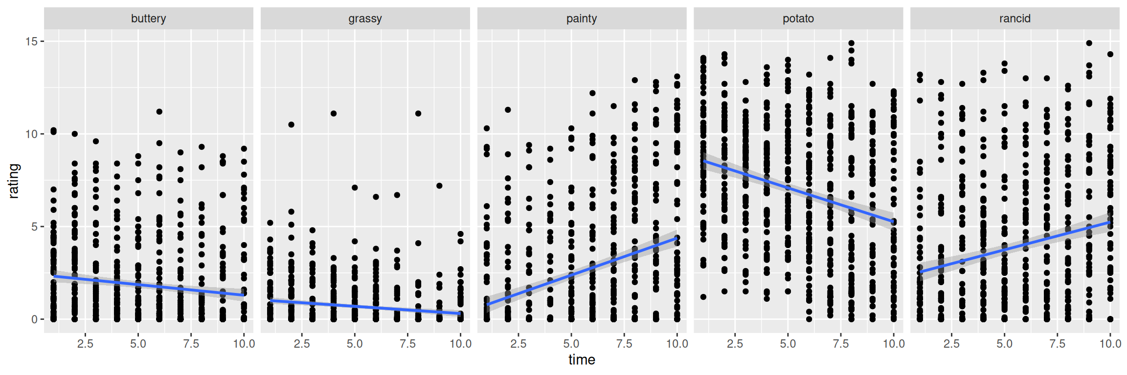

Linear Model

ff_lm <- lm(rating~type-1+as.numeric(time):type, data = ff_long)
summary(ff_lm)

Call:
lm(formula = rating ~ type - 1 + as.numeric(time):type, data = ff_long)

Residuals:
    Min      1Q  Median      3Q     Max 
-7.3463 -1.7771 -0.6146  1.5262 10.6542 

Coefficients:
                             Estimate Std. Error t value Pr(>|t|)    
typebuttery                   2.43478    0.23912  10.182  < 2e-16 ***
typegrassy                    1.08121    0.23907   4.523 6.31e-06 ***
typepainty                    0.38065    0.23909   1.592  0.11146    
typepotato                    8.91167    0.23907  37.276  < 2e-16 ***
typerancid                    2.24631    0.23907   9.396  < 2e-16 ***
typebuttery:as.numeric(time) -0.11416    0.03951  -2.890  0.00388 ** 
typegrassy:as.numeric(time)  -0.07777    0.03945  -1.971  0.04877 *  
typepainty:as.numeric(time)   0.39955    0.03948  10.122  < 2e-16 ***
typepotato:as.numeric(time)  -0.36534    0.03945  -9.261  < 2e-16 ***
typerancid:as.numeric(time)   0.29947    0.03945   7.591 4.06e-14 ***
---
Signif. codes:  0 '***' 0.001 '**' 0.01 '*' 0.05 '.' 0.1 ' ' 1

Residual standard error: 2.935 on 3461 degrees of freedom
  (9 observations deleted due to missingness)
Multiple R-squared:  0.6406,    Adjusted R-squared:  0.6395 
F-statistic: 616.9 on 10 and 3461 DF,  p-value: < 2.2e-16

The Same Linear Model

ff_lm2 <- lm(rating~type*as.numeric(time), data = ff_long)
summary(ff_lm2)

Call:
lm(formula = rating ~ type * as.numeric(time), data = ff_long)

Residuals:
    Min      1Q  Median      3Q     Max 
-7.3463 -1.7771 -0.6146  1.5262 10.6542 

Coefficients:
                            Estimate Std. Error t value Pr(>|t|)    
(Intercept)                  2.43478    0.23912  10.182  < 2e-16 ***
typegrassy                  -1.35357    0.33813  -4.003 6.38e-05 ***
typepainty                  -2.05413    0.33814  -6.075 1.38e-09 ***
typepotato                   6.47690    0.33813  19.155  < 2e-16 ***
typerancid                  -0.18846    0.33813  -0.557  0.57731    
as.numeric(time)            -0.11416    0.03951  -2.890  0.00388 ** 
typegrassy:as.numeric(time)  0.03640    0.05583   0.652  0.51452    
typepainty:as.numeric(time)  0.51372    0.05585   9.198  < 2e-16 ***
typepotato:as.numeric(time) -0.25117    0.05583  -4.499 7.06e-06 ***
typerancid:as.numeric(time)  0.41363    0.05583   7.408 1.60e-13 ***
---
Signif. codes:  0 '***' 0.001 '**' 0.01 '*' 0.05 '.' 0.1 ' ' 1

Residual standard error: 2.935 on 3461 degrees of freedom
  (9 observations deleted due to missingness)
Multiple R-squared:  0.3816,    Adjusted R-squared:   0.38 
F-statistic: 237.3 on 9 and 3461 DF,  p-value: < 2.2e-16

Modelling Treatment

ff_lm_trt <- lm(rating~treatment:(type-1+as.numeric(time):type), 
data=ff_long)

ff_long |> 
  ggplot(aes(x = time, y = rating)) + 
  geom_point() + 
  geom_smooth(aes(colour = treatment), 
              method="lm", se=FALSE, linewidth = 1.5) + 
  facet_grid(~type)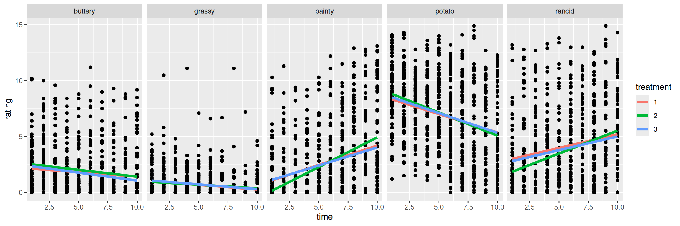

Generally …

Lots of models
summary, str, resid, fitted, coef, … allow us to extract different parts of a model for a linear model. Other model functions work differently … major headaches!

summary(ff_lm)

Call:
lm(formula = rating ~ type - 1 + as.numeric(time):type, data = ff_long)

Residuals:
    Min      1Q  Median      3Q     Max 
-7.3463 -1.7771 -0.6146  1.5262 10.6542 

Coefficients:
                             Estimate Std. Error t value Pr(>|t|)    
typebuttery                   2.43478    0.23912  10.182  < 2e-16 ***
typegrassy                    1.08121    0.23907   4.523 6.31e-06 ***
typepainty                    0.38065    0.23909   1.592  0.11146    
typepotato                    8.91167    0.23907  37.276  < 2e-16 ***
typerancid                    2.24631    0.23907   9.396  < 2e-16 ***
typebuttery:as.numeric(time) -0.11416    0.03951  -2.890  0.00388 ** 
typegrassy:as.numeric(time)  -0.07777    0.03945  -1.971  0.04877 *  
typepainty:as.numeric(time)   0.39955    0.03948  10.122  < 2e-16 ***
typepotato:as.numeric(time)  -0.36534    0.03945  -9.261  < 2e-16 ***
typerancid:as.numeric(time)   0.29947    0.03945   7.591 4.06e-14 ***
---
Signif. codes:  0 '***' 0.001 '**' 0.01 '*' 0.05 '.' 0.1 ' ' 1

Residual standard error: 2.935 on 3461 degrees of freedom
  (9 observations deleted due to missingness)
Multiple R-squared:  0.6406,    Adjusted R-squared:  0.6395 
F-statistic: 616.9 on 10 and 3461 DF,  p-value: < 2.2e-16

Tidying model output

The package broom (broom.mixed for glmmTMB) gets model results into a tidy format at different levels

model level: broom::glance (values such as AIC, BIC, model fit, …)
coefficients in the model: broom::tidy (estimate, confidence interval, significance level, …)
observation level: broom::augment (fitted values, residuals, predictions, influence, …)

Goodness of fit statistics: `glance`

glance(ff_lm)
# A tibble: 1 × 12
  r.squared adj.r.squared sigma statistic p.value    df logLik    AIC    BIC
      <dbl>         <dbl> <dbl>     <dbl>   <dbl> <dbl>  <dbl>  <dbl>  <dbl>
1     0.641         0.640  2.94      617.       0    10 -8658. 17338. 17405.
# ℹ 3 more variables: deviance <dbl>, df.residual <int>, nobs <int>

Model estimates: `tidy`

ff_lm_tidy <- tidy(ff_lm)
head(ff_lm_tidy)
# A tibble: 6 × 5
  term                         estimate std.error statistic   p.value
  <chr>                           <dbl>     <dbl>     <dbl>     <dbl>
1 typebuttery                     2.43     0.239      10.2  5.16e- 24
2 typegrassy                      1.08     0.239       4.52 6.31e-  6
3 typepainty                      0.381    0.239       1.59 1.11e-  1
4 typepotato                      8.91     0.239      37.3  5.41e-256
5 typerancid                      2.25     0.239       9.40 9.98e- 21
6 typebuttery:as.numeric(time)   -0.114    0.0395     -2.89 3.88e-  3

Model diagnostics: `augment`

ff_lm_all <- augment(ff_lm)
glimpse(ff_lm_all)
Rows: 3,471
Columns: 10
$ .rownames          <chr> "1", "2", "3", "4", "5", "6", "7", "8", "9", "10", …
$ rating             <dbl> 2.9, 0.0, 0.0, 0.0, 5.5, 14.0, 0.0, 0.0, 1.1, 0.0, …
$ type               <chr> "potato", "buttery", "grassy", "rancid", "painty", …
$ `as.numeric(time)` <dbl> 1, 1, 1, 1, 1, 1, 1, 1, 1, 1, 1, 1, 1, 1, 1, 1, 1, …
$ .fitted            <dbl> 8.5463333, 2.3206108, 1.0034418, 2.5457779, 0.78019…
$ .resid             <dbl> -5.6463333, -2.3206108, -1.0034418, -2.5457779, 4.7…
$ .hat               <dbl> 0.004876355, 0.004877198, 0.004876355, 0.004876355,…
$ .sigma             <dbl> 2.934289, 2.935600, 2.935817, 2.935546, 2.934764, 2…
$ .cooksd            <dbl> 1.821911e-03, 3.078042e-04, 5.754115e-05, 3.703694e…
$ .std.resid         <dbl> -1.92821044, -0.79248385, -0.34267319, -0.86937756,…

Residual plot

ggplot(ff_lm_all, aes(x=.fitted, y=.resid)) + geom_point()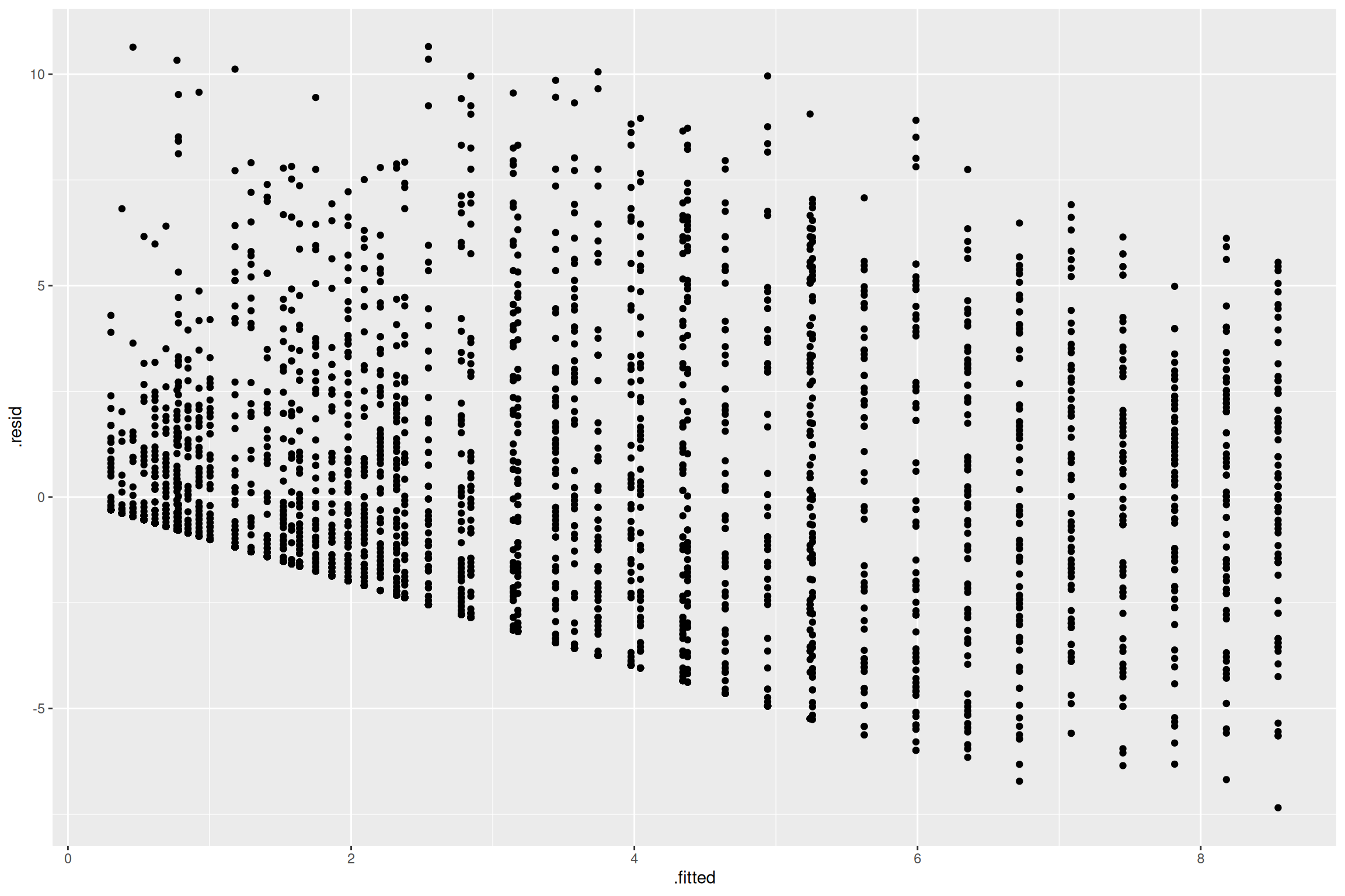

Adding random effects

Add random intercepts for each subject

fries_lmer <- lmer(rating ~ type-1+as.numeric(time):type + ( 1 | subject ), 
data = ff_long)

Your turn

Run the code of the examples so far

The broom.mixed package provides similar functionality to mixed effects models as broom does for fixed effects models

Try out the functionality of broom.mixed on each level: model, parameters, and data
Augment the ff_long data with the model diagnostics
Plot fitted values of the linear model against fitted values of the mixed effects model

References

This work is licensed under a Creative Commons Attribution-NonCommercial-ShareAlike 4.0 International License.

Outline

dplyr verbs

Filter

Arrange

Select

Summarise

Summarise and group_by

Let’s use these tools

Completeness

Your turn

French Fries - completeness

Other nice short cuts

Counts for subject by time

Models and model output

Linear Model

The Same Linear Model

Modelling Treatment

Generally …

Tidying model output

Goodness of fit statistics: glance

Model estimates: tidy

Model diagnostics: augment

Residual plot

Adding random effects

Your turn

References

Goodness of fit statistics: `glance`

Model estimates: `tidy`

Model diagnostics: `augment`

References

- Posit cheatsheets
- Wickham (2007) Reshaping data
- broom vignettes, David Robinson
- Wickham (2011) Split-Apply-Combine