Visual methods for multivariate data - a journey beyond 3D
About the penguins data

|

|
|
| Adélie 1 | Gentoo 2 | Chinstrap 3 |
Simple scatterplot

Our first tour
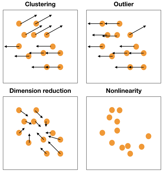
Movement patterns
Movement of points, generally in a grand tour, can provide additional information about structure in high-dimensions.
Reading axes - interpretation
Length and direction of axes relative to the pattern of interest

Reading axes - interpretation
Length and direction of axes relative to the pattern of interest

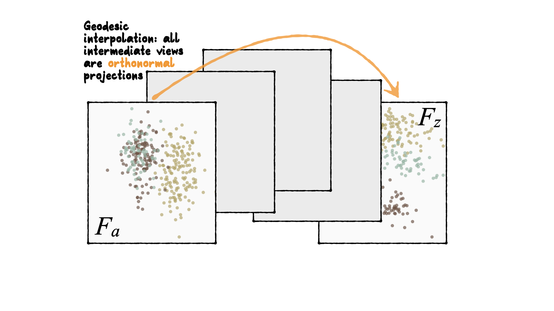
Geodesic interpolation between planes
Tour is indexed by time, \(F(t)\), where \(t\in [a, z]\). Starting and target frame denoted as \(F_a = F(a), F_z=F(t)\).
The animation of the projected data is given by a path \({\mathbf y}_i(t)={\mathbf x}_iF(t)\).
4D spheres
Hollow
Solid
4D cubes
Hollow
Solid
Others
Torus
Mobius
Path on the space of all projections
A grand tour is like a random walk (with interpolation) through the space of all possible projections: sphere for 1D, torus for 2D.1
Grand
Might accidentally see best separation
Guided, using LDA index
Moves to the best separation
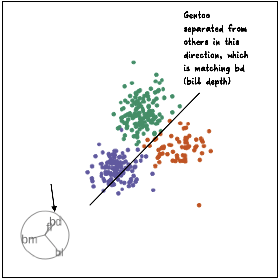
Manual tour
- start from best projection, given by projection pursuit
bdcontribution controlled- if
bdis removed from projection, Gentoo separation disappears bdis important for distinguishing Gentoo

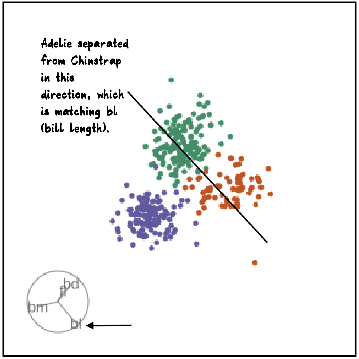
Manual tour
- start from best projection, given by projection pursuit
blcontribution controlledblis important for distinguishing Adelie from Chinstrap
Local tour
Rocks from and to a given projection, in order to observe the neighbourhood
Slice tour
Solid 4D sphere
Hollow 4D sphere
Geometric shapes with slice tour
4D Torus
4D Hollow Cube
PCA tour
Compute PCA, reduce dimension, show original variable axes in the reduced space.
Projection dimension and displays
1D projections displayed as a density
Density contours overlaid on a scatterplot