```{r, include = FALSE}
# Load libraries
source("libraries.R")
# Set up chunk for all slides
source("chunk_options_and_themes.R")
```
## About the presenter
:::: {.columns}
::: {.column style="font-size: 110%; width: 35%;"}
Dianne Cook
*Distinguished Professor*
Monash University
🌐 https://dicook.org/
🦣 @visnut@aus.social
 @visnut.bsky.social
:::
::: {.column style="font-size: 90%; width: 65%;"}
* I have a PhD in Statistics from Rutgers University, NJ, and a Bachelor of Science (Pure Mathematics, Statistics and Biochemistry) from University of New England
* I am a Fellow of the American Statistical Association, elected member of the the R Foundation and International Statistical Institute, Past-Editor of the Journal of Computational and Graphical Statistics, and the R Journal.
* My research is in data visualisation, statistical graphics and computing, with application to sports, ecology and bioinformatics. I like to develop new methodology and software.
* Students in my lab work on methods and software that is generally useful for the world. They have been responsible for bringing you the ggplot2, tidyverse suite, knitr, plotly, and many other R packages are frequently used.
:::
::::
## Got a question, or a comment?
@visnut.bsky.social
:::
::: {.column style="font-size: 90%; width: 65%;"}
* I have a PhD in Statistics from Rutgers University, NJ, and a Bachelor of Science (Pure Mathematics, Statistics and Biochemistry) from University of New England
* I am a Fellow of the American Statistical Association, elected member of the the R Foundation and International Statistical Institute, Past-Editor of the Journal of Computational and Graphical Statistics, and the R Journal.
* My research is in data visualisation, statistical graphics and computing, with application to sports, ecology and bioinformatics. I like to develop new methodology and software.
* Students in my lab work on methods and software that is generally useful for the world. They have been responsible for bringing you the ggplot2, tidyverse suite, knitr, plotly, and many other R packages are frequently used.
:::
::::
## Got a question, or a comment?
✋ 🔡 You can [ask]{.monash-blue2} directly by raising your hand. any time.
[I hope you have many questions!]{.monash-orange2} 🙋🏻👣
## Outline
:::: columns
::: column
- Tidy data
- Organising data into tidy form
- Handling missing values
- Reproducible projects
- Data fusion
:::
::: column
**Everything that you see in these slides can be reproduced using the code embedded in the slides.**
:::
::::
## Follow along
This workshop is designed to provide you with every day tools to improve your data analysis efficiency and effectiveness. All the code and examples to reproduce everything discussed are available at [https://dicook.github.io/BAPPENAS_2025/](https://dicook.github.io/BAPPENAS_2025/)
## What is "big data"?
[*Big data is extremely overhyped and not terribly well defined. Many people think they have big data, when they actually don't.*](https://peadarcoyle.wordpress.com/2015/08/02/interview-with-a-data-scientist-hadley-wickham/) [~Hadley Wickham]{.smallest}
::: {.incremental}
- Big data problems that are actually small data problems, once you have the right subset/sample/summary. ~90%
- Big data problems that are actually lots and lots of small data problems, e.g. you need to fit one model per individual for thousands of individuals. ~9%
- Finally, there are irretrievably big problems where you do need all the data, perhaps because you fitting a complex model.
:::
::: {.fragment}
At least when you first tackle a data problem, after which you might scale up and automate operations.
:::
## Approach {.transition-slide .center style="text-align: center;"}
The methods and tools discussed will ensure you can get started and have a process to follow to develop the appropriate analysis.
## Tidy data {.transition-slide .center style="text-align: center;"}
## Using `tidyr`, `dplyr`
::: columns
::: {.column width="90%"}
- Writing readable code using **pipes**
- What is **tidy data**? Why do you want tidy data? Getting your data into tidy form using tidyr.
- Reading different **data formats**
- String operations, working with **text**
:::
::: {.column width="10%"}


:::
:::
## The pipe operator `%>%` or `|>`
::: columns
::: {.column width="70%"}
- read as `then`
- `x %>% f(y)` and `x |> f(y)` is the same as `f(x, y)`
- `%>%` is part of the `dplyr` package (really, `magrittr`),
`|>` is part of base R
- pipes structure code as *sequence of operations* -- as opposed to function order `g(f(x))`
:::
::: {.column width="30%"}

:::
:::
## The pipe operator `%>%` or `|>`
- `%>%` is part of `dplyr` package (or more precisely, the `magrittr` package)
- R 4.1 introduced the `|>` base pipe (no package necessary)
- An explanation of the (subtle) differences between the pipes can be found [here](https://towardsdatascience.com/understanding-the-native-r-pipe-98dea6d8b61b)
## Pipe Example
::: panel-tabset
### Using `%>%` {-}
```{r read TB incidence data and check, results='hide'}
tb <- read_csv("data/TB_notifications_2025-07-22.csv")
tb %>% # first we get the tb data
filter(year == 2023) %>% # then we focus on the most recent year
group_by(country) %>% # then we group by country
summarize(
cases = sum(c_newinc, na.rm=TRUE) # to create a summary of all new cases
) %>%
arrange(desc(cases)) # then we sort countries to show highest number of new cases first
```
### Using `|>` {-}
```{r read TB incidence data and check base pipe, results='hide'}
tb <- read_csv("data/TB_notifications_2025-07-22.csv")
tb |> # first we get the tb data
filter(year == 2023) |> # then we focus on the most recent year
group_by(country) |> # then we group by country
summarize(
cases = sum(c_newinc, na.rm=TRUE) # to create a summary of all new cases
) |>
arrange(desc(cases)) # then we sort countries to show highest number new cases first
```
:::
```{r show-results, echo=FALSE}
tb <- read_csv("data/TB_notifications_2025-07-22.csv")
tb |> # first we get the tb data
filter(year == 2023) |> # then we focus on the most recent year
group_by(country) |> # then we group by country
summarize(
cases = sum(c_newinc, na.rm=TRUE) # to create a summary of all new cases
) |>
arrange(desc(cases)) # then we sort countries to show highest number of new cases first
```
## What is tidy data?
::: columns
::: {.column width="60%"}
{width="100%"}
[Illustrations from the Openscapes blog Tidy Data for reproducibility, efficiency, and collaboration by [Julia Lowndes and Allison Horst](https://allisonhorst.com/other-r-fun)]{.smallest}
:::
::: {.column width="40%"}
- What do we expect tidy data to look like?
- maybe easier: what are sources of messiness?
:::
:::
## Varying degree of messiness
::: panel-tabset
### Cryptic Names
What are the variables? Where are they located?
```{r example 1 What are the variables, echo=FALSE}
grad <- read_csv("data/graduate-programs.csv")
head(grad[c(2,3,4,6)])
```
::: notes
in the columns, subject, Inst, AvNumPubs, ...
:::
### More cryptic
What's in the column names of this data? What are the experimental units? What are the measured variables?
```{r example 2 whats in the column names, echo=FALSE}
genes <- read_csv("data/genes.csv")
head(genes)
```
::: notes
the experimental design is coded into the variable names, genotype:WI/WM, time:6/12, rep:1/2/4
:::
### Most
What are the variables? What are the records?
```{r example 3 what are the variables and records, echo=FALSE}
melbtemp <- read.fwf("data/ASN00086282.dly",
c(11, 4, 2, 4, rep(c(5, 1, 1, 1), 31)), fill=T)
head(melbtemp[,c(1,2,3,4,seq(5,100,4))])
```
::: notes
variables are TMAX, TMIN, PRCP, year, month, day, stationid.
Each row contains the values for one month!
:::
### Too_much_info
What are the variables? What are the experimental units?
```{r example 4 what are the variables and experimental units, echo=FALSE}
tb <- read_csv("data/tb.csv")
tail(tb)
#colnames(tb)
```
### Tables
What are the variables? What are the observations?
```{r example 4 what are the variables and observations, echo=FALSE}
pew <- read.delim(
file = "http://stat405.had.co.nz/data/pew.txt",
header = TRUE,
stringsAsFactors = FALSE,
check.names = F
)
pew[1:5, 1:5]
```
### Gross on repeat
10 week sensory experiment, 12 individuals assessed taste of french fries on several scales (how potato-y, buttery, grassy, rancid, paint-y do they taste?), fried in one of 3 different oils, replicated twice.
First few rows:
```{r example 6 what are the factors measurements and experimental units, echo = FALSE}
load("data/french_fries.rda")
head(french_fries, 4)
```
What is the experimental unit? What are the factors of the experiment? What was measured? What do you want to know?
:::
## Messy data patterns
There are various features of messy data that one can observe in practice. Here are some of the more commonly observed patterns:
- Column headers are not just variable names, but also contain values
- Variables are stored in both rows and columns, contingency table format
- One type of experimental unit stored in multiple tables
- Dates in many different formats
## Tidy Data Conventions
1. Data is contained in a single table
2. Each observation forms a row (no data info in column names)
3. Each variable forms a column (no mashup of multiple pieces of information)
## Long and Wide
- Long form: **one** measured value per row. All other variables are descriptors (key variables) - good for modelling, terrible for most other analyses, e.g. correlation matrix
- Widest form: **all** measured values for an entity are in a single row.
- Wide form: measurements are arranged by *some of the descriptors* in columns (for direct comparisons)
##
{width=80%}
[Illustrations from the Openscapes blog: Tidy Data for reproducibility, efficiency, and collaboration by [Julia Lowndes and Allison Horst](https://allisonhorst.com/other-r-fun)]{.smallest}
## Tidy verbs
- `pivot_longer`: get information out of names into columns
- `pivot_wider`: make columns of observed data for levels of design variables (for comparisons)
- `separate`/`unite`: split and combine columns
- `nest`/`unnest`: make/unmake variables into sub-data frames of a list variable
## Pivot to long form
::: columns
::: {.column width=70%}
```
data |> pivot_longer(cols, names_to = "name", values_to = "value", ...)
```
- `pivot_longer` turns a wide format into a long format
- two new variables are introduced (in key-value format): **name** and **value**
- `col` defines which variables should be combined
:::
::: {.column width=30%}
[tidyr cheat sheet](https://rstudio.github.io/cheatsheets/tidyr.pdf)
](https://github.com/gadenbuie/tidyexplain/raw/main/images/tidyr-pivoting.gif)
:::
:::
## Pivoting: an example
```{r setup a simple example, echo = FALSE}
dframe <- data.frame(id = 1:2, trtA=c(2.5,4.6), trtB = c(45, 35))
```
```{r gather the example data into long form}
# wide format
dframe
# long format
dframe |> pivot_longer(trtA:trtB, names_to="treatment", values_to="outcome")
```
## Variable selectors
- `data |> pivot_longer(cols, names_to = "key", values_to = "value", ...)`
- `cols` argument identifies variables that should be combined.
- **Pattern Selectors** can be used to identify variables by **name**, **position**, a range (using `:`), a pattern, or a combination of all.
## Examples of pattern selectors
- `starts_with(match, ignore.case = TRUE, vars = NULL)`
- other select functions: `ends_with`, `contains`, `matches`.
- For more details, see `?tidyselect::language`
## TB notifications
New notifications of TB have the form `new_sp_`:
```{r read in and process the TB data}
read_csv("data/TB_notifications_2025-07-22.csv") |>
dplyr::select(country, iso3, year, starts_with("new_sp_")) |>
na.omit() |>
head()
```
## Pivot longer: TB notifications
create two new variables: `name` and `value`
- `name` contains all variable names starting with "new_sp_"
- `value` contains all values of the selected variables
```{r turn TB data into long form}
tb1 <- read_csv("data/TB_notifications_2025-07-22.csv") |>
dplyr::select(country, iso3, year, starts_with("new_sp_")) |>
pivot_longer(starts_with("new_sp_"))
tb1 |> na.omit() |> head()
```
## Separate columns
```
data |> separate_wider_delim (col, delim, names, ...)
```
- split column `col` from data frame `frame` into a set of columns as specified in `names`
- `delim` is the delimiter at which we split into columns, splitting separator.
## Separate TB notifications
Work on `name`:
```{r extract variable names from original column names}
tb2 <- tb1 |>
separate_wider_delim(
name, delim = "_",
names=c("toss_new", "toss_sp", "sexage"))
tb2 |> na.omit() |> head()
```
## Separate columns
`data %>% separate_wider_position(col, widths, ...)`
- split column `col` from `frame` into a set of columns specified in `widths`
- `widths` is named numeric vector where the names become column names; unnamed components will be matched but not included.
## Separate TB notifications again
Now split `sexage` into first character (m/f) and rest.
```{r continue extracting variable names}
tb3 <- tb2 %>% dplyr::select(-starts_with("toss")) |> # remove the `toss` variables
separate_wider_position(
sexage,
widths = c(sex = 1, age = 4),
too_few = "align_start"
)
tb3 |> na.omit() |> head()
```
The data could be made prettier but it is now in form that can be analysed with standard handling.
## Try this one
Read the genes data from folder `data`. Column names contain data and are kind of messy.
```{r}
genes <- read_csv("data/genes.csv")
names(genes)
```
Produce the data frame called `gtidy` as shown below:
```{r}
#| label: code solution to genes wrangling
#| code-fold: true
gtidy <- genes |>
pivot_longer(-id, names_to="variable", values_to="expr") |>
separate_wider_delim(variable, names=c("trt", "leftover"),
delim = "-") |>
separate_wider_delim(leftover, names=c("time", "rep"),
delim = ".") |>
mutate(trt = sub("W", "", trt)) |>
mutate(rep = sub("R", "", rep))
```
```{r}
head(gtidy)
```
## Plot the genes data overlaid with group means
::: columns
::: column
```{r compute group means, fig.show='hide'}
gmean <- gtidy |>
group_by(id, trt, time) |>
summarise(expr = mean(expr))
gtidy |>
ggplot(aes(x = trt, y = expr, colour=time)) +
geom_point() +
geom_line(data = gmean, aes(group = time)) +
facet_wrap(~id) +
scale_colour_brewer("", palette="Set1")
```
:::
::: column
```{r plot the genes data overlaid with group means, echo=FALSE, fig.width=5, fig.height = 5}
gtidy |>
ggplot(aes(x = trt, y = expr, colour=time)) +
geom_point() +
geom_line(data = gmean, aes(group = time)) +
facet_wrap(~id) +
scale_colour_brewer("", palette="Set1")
```
:::
:::
## {.information-slide .center style="text-align: center;"}
Getting data into tidy form is the singularly most efficient and generalisable way to do data analysis
## Initial data analysis (IDE) {.transition-slide .center style="text-align: center;"}
## Objectives
The [**main objective for IDA**]{.monash-blue2} is to intercept any problems in the data that might adversely affect the confirmatory data analysis.
**_IDA is often unreported_** in the data analysis reports or scientific papers, for various reasons. It might not have been done, or it may have been conducted but there was no space in the paper to report on it.
[**Good practice**]{.monash-blue2} expects that this work is transparent and repeatable and changeable.
## Data cleaning
The purpose of [data cleaning]{.monash-blue2} is to bring data up to a level of quality such that it can reliably be used for the production of statistical models or statements.
A [statistical value chain]{.monash-blue2} is constructed by defining a number of meaningful intermediate data products, for which a chosen set of quality attributes are well described.
{width="500px" fig-align="center"}
[Data cleaning in Government Statistics: van der Loo & de Jonge (2018) Statistical Data Cleaning with Applications in R]{.smallest}
## Data screening
:::: {.columns}
::: {.column width=50%}
::: {.info}
It's important to check how the data are [understood by the computer]{.monash-blue2}.
:::
that is, checking for _data type_:
* Was the date read in as character?
* Was a factor read in as numeric?
:::
::: {.column width=50%}
```{r, echo = FALSE}
xlsx_df <- read_excel("data/lecture3-example.xlsx",
col_types = c("text", "date", "text", "numeric")) |>
mutate(id = as.factor(id),
date = as.character(date),
date = as.Date(date, format = "%Y-%d-%m"))
```
You can visualise the data type with the `visdat` package:
```{r echo = TRUE}
vis_dat(xlsx_df)
```
:::
::::
## Example: Checking the data type [(1/2)]{.smallest}
:::: {.columns}
::: {.column width=50%}
`lecture3-example.xlsx`
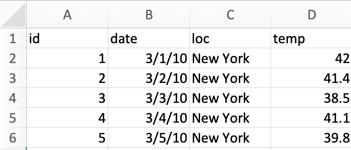 :::
::: {.column width=50%}
```{r, echo = TRUE}
df <- read_excel("data/lecture3-example.xlsx")
df
```
- What problems are there with the computer's interpretation of [data type]{.monash-orange2}?
- What [context]{.monash-orange2} specific issues indicate incorrect computer interpretation?
:::
::::
## Example: Checking the data type [(2/2)]{.smallest}
:::: {.columns}
::: {.column width=50%}
```{r, echo = TRUE}
df <- read_excel("data/lecture3-example.xlsx",
col_types = c("text",
"date",
"text",
"numeric"))
df |>
mutate(id = as.factor(id),
date = ydm(date)) |>
mutate(
day = day(date),
month = month(date),
year = year(date))
```
:::
::: {.column width=50%}
* `id` is now a `factor` instead of `integer`
* `day`, `month` and `year` are now extracted from the `date`
* Is it okay now?
::: {style="font-size: 70%;"}
::: {.fragment}
* In the United States, it's common to use the date format MM/DD/YYYY (gasps) while the rest of the world commonly uses DD/MM/YYYY or better still YYYY/MM/DD.
:::
::: {.fragment}
* It's highly probable that the dates are 1st-5th March and not 3rd of Jan-May.
:::
::: {.fragment}
* You can validate interpretation of temperature using [weather database](https://www.wunderground.com/history/monthly/us/ny/new-york-city/KLGA/date/2010-3).
:::
:::
:::
::::
## Handling missing values {.transition-slide .center style="text-align: center;"}
## Case study: World development indicators [(1/7)]{.smallest}
:::: {.columns}
::: {.column width=70%}
```{r}
options(width=80)
raw_dat <- read_csv("data/world-development-indicators.csv",
na = "..", n_max = 11935)
glimpse(raw_dat)
```
[World Development Indicators (WDI), sourced from the [World Bank Group (2019)](https://databank.worldbank.org/source/world-development-indicators/)]{.smallest}
:::
::: {.column width=30%}
:::
::: {.column width=50%}
```{r, echo = TRUE}
df <- read_excel("data/lecture3-example.xlsx")
df
```
- What problems are there with the computer's interpretation of [data type]{.monash-orange2}?
- What [context]{.monash-orange2} specific issues indicate incorrect computer interpretation?
:::
::::
## Example: Checking the data type [(2/2)]{.smallest}
:::: {.columns}
::: {.column width=50%}
```{r, echo = TRUE}
df <- read_excel("data/lecture3-example.xlsx",
col_types = c("text",
"date",
"text",
"numeric"))
df |>
mutate(id = as.factor(id),
date = ydm(date)) |>
mutate(
day = day(date),
month = month(date),
year = year(date))
```
:::
::: {.column width=50%}
* `id` is now a `factor` instead of `integer`
* `day`, `month` and `year` are now extracted from the `date`
* Is it okay now?
::: {style="font-size: 70%;"}
::: {.fragment}
* In the United States, it's common to use the date format MM/DD/YYYY (gasps) while the rest of the world commonly uses DD/MM/YYYY or better still YYYY/MM/DD.
:::
::: {.fragment}
* It's highly probable that the dates are 1st-5th March and not 3rd of Jan-May.
:::
::: {.fragment}
* You can validate interpretation of temperature using [weather database](https://www.wunderground.com/history/monthly/us/ny/new-york-city/KLGA/date/2010-3).
:::
:::
:::
::::
## Handling missing values {.transition-slide .center style="text-align: center;"}
## Case study: World development indicators [(1/7)]{.smallest}
:::: {.columns}
::: {.column width=70%}
```{r}
options(width=80)
raw_dat <- read_csv("data/world-development-indicators.csv",
na = "..", n_max = 11935)
glimpse(raw_dat)
```
[World Development Indicators (WDI), sourced from the [World Bank Group (2019)](https://databank.worldbank.org/source/world-development-indicators/)]{.smallest}
:::
::: {.column width=30%}
- What are the data types?
- What are the variables?
- What are the observations?
- Is the data in tidy form?
:::
::::
## Case study: World development indicators [(2/7)]{.smallest}
:::: {.columns}
::: {.column width=60%}
```{r}
country_code_df <- raw_dat |>
distinct(`Country Name`, `Country Code`) |>
rename_all(janitor::make_clean_names) |>
left_join(
countrycode::codelist |> select(iso3c, region, continent),
by = c("country_code" = "iso3c")
) |>
arrange(continent, region)
```
::: {style="font-size: 70%;"}
```{r}
#| echo: false
options(width=80)
glimpse(country_code_df)
country_code_df |> count(continent)
country_code_df |> count(region)
```
:::
:::
::: {.column width=40%}
- How many countries are included
- How many continents, regions?
- Why are there NAs here?
::: {.fragment style="font-size: 70%;"}
```{r}
country_code_df |> filter(is.na(continent))
```
:::
:::
::::
## Case study: World development indicators [(3/7)]{.smallest}
:::: {.columns}
::: {.column width=60%}
```{r}
wdi_vars <- raw_dat |>
select(`Series Name`, `Series Code`) |>
distinct() |>
rename_all(janitor::make_clean_names)
```
::: {style="font-size: 60%; overflow: auto; max-height: 650px;"}
```{r}
#| echo: false
wdi_vars |> gt::gt()
```
:::
:::
::: {.column width=40%}
- Analysis will use the short name (`series_code`) for variables.
- Store full variable name (`series_name`) and short name (`series_code`) in a separate table.
- The `series_code` will be used as the key whenever the full name is needed.
:::
::::
## Case study: World development indicators [(4/7)]{.smallest}
:::: {.columns}
::: {.column width=50%}
```{r}
wdi <- raw_dat |>
select(`Country Code`, `Series Code`, `1969 [YR1969]`:`2018 [YR2018]`) |>
rename_all(janitor::make_clean_names) |>
pivot_longer(x1969_yr1969:x2018_yr2018,
names_to = "year",
values_to = "value") |>
mutate(year = as.numeric(str_sub(year, 2, 5)) ) |>
pivot_wider(names_from = series_code,
values_from = value)
wdi2017 <- wdi |> filter(year == 2017)
```
- Organise data into tidy form
- Check missing value distribution
:::
::: {.column width=50%}
```{r}
#| fig-width: 8
#| fig-height: 7
#| code-fold: true
vis_miss(wdi, sort_miss = TRUE)
```
:::
::::
## Case study: World development indicators [(5/7)]{.smallest}
:::: {.columns}
::: {.column width=20%}
Check missings by
- variable
- country
:::
::: {.column width=50%}
```{r}
#| fig-width: 8
#| fig-height: 6
#| code-fold: true
gg_miss_var(wdi, show_pct=TRUE)
```
:::
::: {.column width=30%}
```{r}
#| code-fold: true
#| fig-width: 2
#| fig-height: 8
#| out-width: 100%
wdi_cnt_miss <- wdi |>
filter(!is.na(country_code)) |>
bind_shadow() |>
select(country_code, year,
SP.ADO.TFRT_NA:SP.URB.GROW_NA) |>
pivot_longer(SP.ADO.TFRT_NA:SP.URB.GROW_NA,
names_to="var",
values_to="value") |>
group_by(country_code) |>
count(value) |>
mutate(value = fct_recode(value,
miss="NA",
not="!NA")) |>
pivot_wider(names_from = value, values_from = n) |>
mutate(p_miss = miss/(miss+not)) |>
select(country_code, p_miss)
wdi_cnt_p <- wdi_cnt_miss |>
ggplot(aes(x=1, y=p_miss,
label=country_code)) +
geom_quasirandom() +
ylim(c(0,1)) + ylab("Prop miss")
ggplotly(wdi_cnt_p)
```
:::
::::
## Case study: World development indicators [(6/7)]{.smallest}
:::: {.columns}
::: {.column width=50%}
Look at Costa Rica (CRI), most complete country
```{r}
#| fig-width: 8
#| fig-height: 6
#| code-fold: true
wdi_cri <- wdi |>
filter(country_code == "CRI")
vis_miss(wdi_cri, sort_miss=TRUE)
```
:::
::: {.column width=50%}
To illustrate imputation, we'll show one of the variables, that is relatively complete.
```{r}
#| fig-width: 6
#| fig-height: 3
#| code-fold: true
wdi_cri_p <- wdi_cri |>
ggplot(aes(x=year, y=SE.PRM.CMPT.ZS)) +
geom_miss_point() +
theme(aspect.ratio=0.5,
legend.position = "none")
wdi_cri_p
```
Impute a few temporal missings using nearest neighbours.
:::
:::
## Case study: World development indicators [(6/7)]{.smallest}
:::: {.columns}
::: {.column width=50%}
Missings imputed using `imputeTS` using the moving average method.
```{r}
#| fig-width: 6
#| fig-height: 3
#| code-fold: true
wdi_cri_v1 <- wdi_cri |>
mutate(SE.PRM.CMPT.ZS = na_ma(SE.PRM.CMPT.ZS))
wdi_cri_v1 |>
ggplot(aes(x=year, y=SE.PRM.CMPT.ZS)) +
geom_point() +
geom_smooth(se=F, colour="#D55E00") +
theme(aspect.ratio=0.5)
```
:::
::: {.column width=50%}
- Don't have to impute before scrutinizing data
- What are these numbers supposed to be?
`SE.PRM.CMPT.ZS` is "Primary completion rate, total (% of relevant age group)"
[Do we have any problems?]{.monash-orange2}
::: {.fragment}
Yes. The explanation of the variable suggests the numbers should range between 0-100.
:::
:::
:::
## Reproducibility, workflow and versioning {.transition-slide .center style="text-align: center;"}
## Dynamic documents
- **Efficiency**: allow changes to be implemented more easily, especially for dynamic reproducible documents.
- **Repeatability**: the analysis can be repeated multiple times while still obtaining the same results.
- **Transparency**: everything is available for access, resulting in more trustworthy results.
- **Easy to update**: when new data arrives, the report can be automatically updated.
::: {.fragment}
These slides are an example of a dynamic document. You can extract the code and re-run all the examples. *What I show you, you can do to.*
:::
## How might the project look?
{width="60%" fig-align="center"}
::: {.smallest}
[Source: Julia Lowndes, useR! 2019 keynote](https://openscapes.org/blog/2019-08-22-user-keynote/)
:::
## How to combine text and data analysis?
::: {.callout-note}
## Literate programming
Literate programming is an approach to writing reports using software that weaves together the source code and text at the time of creation.
:::
::: {.smaller}
Reproducibility requires more than literate programming. These are:
- a versioning and sharing system, like GitHub and git.
- software environment supporting workflows such as [targets](https://docs.ropensci.org/targets/) or [renv](https://rstudio.github.io/renv/articles/renv.html).
:::
## Getting started {.transition-slide .center style="text-align: center;"}
## [First step]{style="color:#006DAE;"}
:::{.callout-caution}
## Practicing
1. Create a project.
2. Create a quarto document.
3. Render document.
:::
## Elements of a reproducible project
- All the elements of the project should be files.
- All files should be stored within the project location (typically a folder).
- All files should be explicitly tied together.
:::{.fragment}
But how do we tie the files together?
:::
## Computer paths
A path is the complete location or name of where a computer file, directory, or web page is located.
Examples:
- `Windows: C:\\Documents\\workshop`
- `Mac/Linux: /Users/Documents/workshop`
- `Internet: https://numbat.space/`
::: {.fragment}
Because these are different on different systems, you should avoid complications and use **relative** paths,
```
raw_dat <- read_csv("data/world-development-indicators.csv",
na = "..", n_max = 11935)
```
From my current directory/folder, find the `data` folder and you will find the file `world-development-indicators.csv`.
:::
## Work projects
- `data` folder: contains all the data for the project.
- `images`/`figures` folder**: contains all the external pictures not produced by the code in the qmd file.
- `.Rproj` file: automatically added when creating an RStudio project (handles the relative paths and working directories).
- `qmd` file: quarto document
- Other `R` scripts, etc...

## Quarto details {.transition-slide .center style="text-align: center;"}
## Quarto
- Provides a framework for integrating code and text into a single document.
- The code is written within the code chunks, put the text around that, and get a fully reproducible document.
{fig-align="center" width="20%" height="20%"}
::: {.smallest}
[Source: GitHub - RStudio hex stickers](https://github.com/rstudio/hex-stickers)
:::
## Quarto document elements
1. **Text** (formatted with Markdown)
2. **Code** (code formatting)
3. **Metadata** (YAML)
{fig-align="center"}
::: {.smallest}
[Source: Quarto Cheatsheets](https://rstudio.github.io/cheatsheets/quarto.pdf)
:::
## Quarto: text (Markdown)
Markdown is a lightweight markup language for adding formatting elements to plain text documents.
- Text formatting
- Headings
- Links & Images
- Lists
- Many more...
## Text formatting & Headings
:::: {.columns}
::: {.column width="50%"}
Markdown Syntax:
```markdown
*italics*, _italics_
**bold**, __bold__
***bold italics***, ___bold italics___
~~strikethrough~~
`verbatimcode`
# Heading 1
## Heading 2
```
:::
::: {.column width="50%"}
Results:
::: {.smaller}
*italics*, _italics_
**bold**, __bold__
***bold italics***, ___bold italics___
~~strikethrough~~
`verbatimcode`
:::
### Heading 1
#### Heading 2
:::
::::
## Links, Images, and Lists
:::: {.columns}
::: {.column width="50%"}
Markdown Syntax:
```markdown
[More quarto](https://quarto.org)

* unordered list
1. ordered list
```
:::
::: {.column width="50%"}
Results:
::: {.smaller}
[More quarto](https://quarto.org)
{width="20%" fig-align="left"}
* unordered list
1. ordered list
:::
:::
::::
## Quarto: code (R)
:::: {.columns}
::: {.column width="50%"}
R code:
````
```
#| echo: false
1+1
```
````
:::
::: {.column width="50%"}
Results:
```{r}
#| echo: false
1 + 1
```
:::
::::
Insert an R code chunk into a Quarto document with:
- Keyboard short cut Ctrl + Alt + I (Mac: Cmd + Option + I)
- Typing the chunk delimiters (```)
Chunk output can be customised with **Chunk execution options**, which are at the top of a chunk, starting with `#|`
## Chunk execution options
- `eval: false` does not evaluate (run) this code chunk when knitting.
- `echo: false` does not show the source code in the finished file.
- `include: false` prevents code and results from showing in the finished file.
- `message: false` prevents messages that are generated by code from showing in the finished file.
- `warning: false` prevents warnings that are generated from showing in the finished file
- `fig.cap = "Text"` adds a caption to a figure
There are many more; see Quarto documentation.
## Tables and captions
:::: {.columns}
::: {.column width="50%"}
R code:
````
```
#| echo: false
library(ggplot2)
data(cars)
table_data <- head(cars, 5)
knitr::kable(table_data,
caption = "Speed and stopping
distances of cars")
```
````
:::
::: {.column width="50%"}
Results:
::: {width="50%"}
```{r}
#| echo: false
library(ggplot2)
data(cars)
table_data <- head(cars, 5)
knitr::kable(table_data,
caption = "Speed and stopping
distances of cars") |>
kableExtra::kable_paper(
full_width = TRUE
)
```
:::
:::
::::
## Figures and captions
:::: {.columns}
::: {.column width="50%"}
R code:
````
```
#| label: cars-plot
#| fig-cap: "Distance taken for a car to stop, against it's speed during the test."
library(ggplot2)
ggplot(cars,
aes(x = speed,
y = dist)
) +
geom_point()
```
````
:::
::: {.column width="50%"}
Results:
::: {width="50%"}
```{r}
#| label: cars-plot
#| fig-cap: "Distance taken for a car to stop, against it's speed during the test."
#| fig-height: 3
library(ggplot2)
ggplot(cars,
aes(x = speed,
y = dist)
) +
geom_point()
```
:::
:::
::::
## Quarto: YAML
Basic YAML syntax
```yaml
title: "My report"
author: "Krisanat A."
format:
html:
toc: true
theme: solar
pdf:
toc: true
```
## Output to different formats, inc Word, PPT
:::: {.columns}
::: {.column width=50%}
**HTML**
{fig-align="center"}
:::
::: {.column width=50%}
**PDF**
{fig-align="center"}
:::
::::
## Quarto templates {.transition-slide .center style="text-align: center;"}
## What is a quarto template?
The templates provide a straightforward way to get started with new Quarto projects by providing example content and options.
:::{.incremental}
1. Create a working initial document for custom formats
2. Provide the initial content for a custom project type
:::
:::{.fragment}
Remember all the painstaking work we did earlier, setting YAML, creating all the folders, and setting the execution options.
:::
:::{.fragment}
All of that can be gone with one line in the terminal!!
:::
## 📚 Adding a Bibliography to `.qmd` Files
````markdown
### 1. Create a `.bib` File (BibTeX Format)
```bibtex
@article{smith2021,
title = {A Method for Data Analysis},
author = {Smith, Jane},
journal = {Journal of Statistics},
year = {2021}
}
````
💡 Save as: `references.bib`
### 1. Link the `.bib` File in YAML
```yaml
bibliography: references.bib
csl: apa.csl # Optional: adds citation style (e.g., APA, IEEE)
```
### 2. Cite in the Text
```markdown
As shown in recent work [@smith2021], the method is effective.
```
🔄 Quarto will automatically format the in-text citation and generate a reference list.
## ⚙️ Quarto quirks & power tips
:::: {.columns}
::: {.column}
📐 LaTeX equation in a figure caption
```markdown
{#fig-einstein}
```
✅ You can embed LaTeX-style equations directly using dollar signs (`$...$`) in the caption.
✅ Works in both **HTML** and **PDF** outputs.
::: {.fragment}
Refer to another figure in a caption
```markdown
{#fig-compare}
```
📝 `@fig-einstein` will resolve to the numbered figure reference (e.g., *Figure 1*) in PDF/HTML.
📌 Make sure the first figure has an ID like `{#fig-einstein}`.
:::
:::
::: {.column}
::: {.fragment}
🔗 Hyperlink in a table
```markdown
| Tool | Link |
|--------|-----------------------------------|
| Quarto | [quarto.org](https://quarto.org) |
```
✅ Use standard Markdown syntax inside tables: `[text](url)`
✅ Works for **external links**, local files, and section anchors.
:::
::: {.fragment}
🖼 Alt-Text in Figure Chunk
```markdown
{fig-alt="A scatterplot showing car stopping distances by speed."}
```
✅ Use `fig-alt="..."` to improve **accessibility** and support screen readers.
:::
:::
::::
## {.information-slide .center style="text-align: center;"}
Open-source software is the powerhouse of our generation. Almost anything that you need to do with data, can be accomplished.
## Data fusion {.transition-slide .center style="text-align: center;"}
## Case study 1: Australian bushfires [1/3]{.smallest}
:::: columns
::: column
Find all the code and data for this work at [https://github.com/TengMCing/bushfire-paper](https://github.com/TengMCing/bushfire-paper)
**Purpose**: Predict the cause of bushfire ignitions in the catastrophic 2019-2020 season for Victoria.
**Model**: random forest trained on historical cause data and linked data on climate, vegetation, distance from roads, campsites, fire stations
**Data linked**: by geographic location of fires
:::
::: column
::: {.fragment style="font-size: 70%;"}
Data sourced from
- Hotspot data from the Himawari-8 satellite
- Climate data from Bureau of Meteorology
(BOM) and Commonwealth Scientific and Industrial Research Organisation (CSIRO)
- road map from a comprehensive open-source map Openstreetmap
- vegetation from Australian Bureau of Agricultural and Resource Economics and Sciences
- **historical fire origins (causes)**, fire stations and camping location from Department of
Environment, Land, Water & Planning.
:::
:::
::::
## Case study 1: Australian bushfires [2/3]{.smallest}
{fig-align="center"}
## Case study 1: Australian bushfires [3/3]{.smallest}
The app is at [https://ebsmonash.shinyapps.io/VICfire/](https://ebsmonash.shinyapps.io/VICfire/).
```{r out.width="110%", echo=FALSE}
knitr::include_app("https://ebsmonash.shinyapps.io/VICfire/", height = "550px")
```
## Case study 2: Australian ecotourism
:::: {.columns}
::: {.column width=40%}
::: {style="font-size: 70%;"}
*Source*: [https://github.com/vahdatjavad/ecotourism](https://github.com/vahdatjavad/ecotourism)
See the R package `ecotourism` on CRAN.
*Data*:
- **Atlas of Living Australia** occurrences of mantaray, glow worms, Gouldian finch and orchids
- Regional records of **Australian tourism** quarterly summaries
- **Weather** downloaded using the GSODR R package.
:::
:::
::: {.column width=60%}

:::
::::
## {.information-slide .center style="text-align: center;"}
Open data is a golden resource for understanding the world around us.
## Resources
::: {style="font-size: 70%;"}
- [R for Data Science (2e)](https://r4ds.hadley.nz)
- [The tidy tools manifesto](https://cran.r-project.org/web/packages/tidyverse/vignettes/manifesto.html)
- [Posit cheatsheets](https://posit.co/resources/cheatsheets/)
- [Wickham (2007) Reshaping data](https://www.jstatsoft.org/article/view/v021i12)
- [van der Loo and de Jonge (2018). Statistical Data Cleaning with Applications in R](https://onlinelibrary.wiley.com/doi/book/10.1002/9781118897126)
- Templates for monash thesis and other documents are [available here](https://github.com/quarto-monash).
- GitHub/git for collaborative and versioned work, start with [Happy Git and GitHub for the useR](https://happygitwithr.com)
- Material on reproducibility and collaboration adapted from workshop by Jayani Lakshika and Krisanat Anukarnsakulchularp.
:::
::: bottom
 This work is licensed under a Creative Commons Attribution-NonCommercial-ShareAlike 4.0 International License.
:::
This work is licensed under a Creative Commons Attribution-NonCommercial-ShareAlike 4.0 International License.
:::