Check distributional assumptions using histograms and the lineup protocol.

This function is used to quickly create lineup plots to check distributional assumptions using histograms with kernel density estimates. The null hypothesis is that the data follows the distribution specified by the dist argument. In the lineup protocol the plot of the real data is embedded amongst a field of plots of data generated to be consistent with some null hypothesis. If the observer can pick the real data as different from the others, this lends weight to the statistical significance of the structure in the plot. The protocol is described in Buja et al. (2009).

lineup_histograms(
  data,
  variable,
  dist = NULL,
  params = NULL,
  color_bars = "black",
  fill_bars = "grey",
  color_lines = "brown3"
)

Arguments

data

a data frame.

variable

the name of the variable that should be plotted.

dist

the null distribution name. One of: "beta", "cauchy", "chi-squared", "exponential", "f", "gamma", "geometric", "log-normal", "lognormal", "logistic", "negative binomial", "binomial", "normal", "poisson", "t", "uniform", "weibull"

params

list of parameters of distribution. If NULL, will use fitdistr to estimate them if possible. For uniform, beta, and binomial distributions, the parameters must be specified. See ?dunif, ?dbeta, and ?dbinom for parameter names.

color_bars

the color used for the borders of the bars. Can be a name or a color HEX code.

fill_bars

the color used to fill the bars.

color_lines

the color used for the density curves.

Value

a ggplot

Details

19 null datasets are plotted together the the true data (randomly positioned) If you pick the real data as being noticeably different, then you have formally established that it is different to with p-value 0.05.

Run the decrypt message printed in the R Console to see which plot represents the true data.

References

Buja, Cook, Hofmann, Lawrence, Lee, Swayne, Wickham. (2009). Statistical inference for exploratory data analysis and model diagnostics, Phil. Trans. R. Soc. A, 367, 4361-4383.

See also

null_dist

Examples

data(tips)
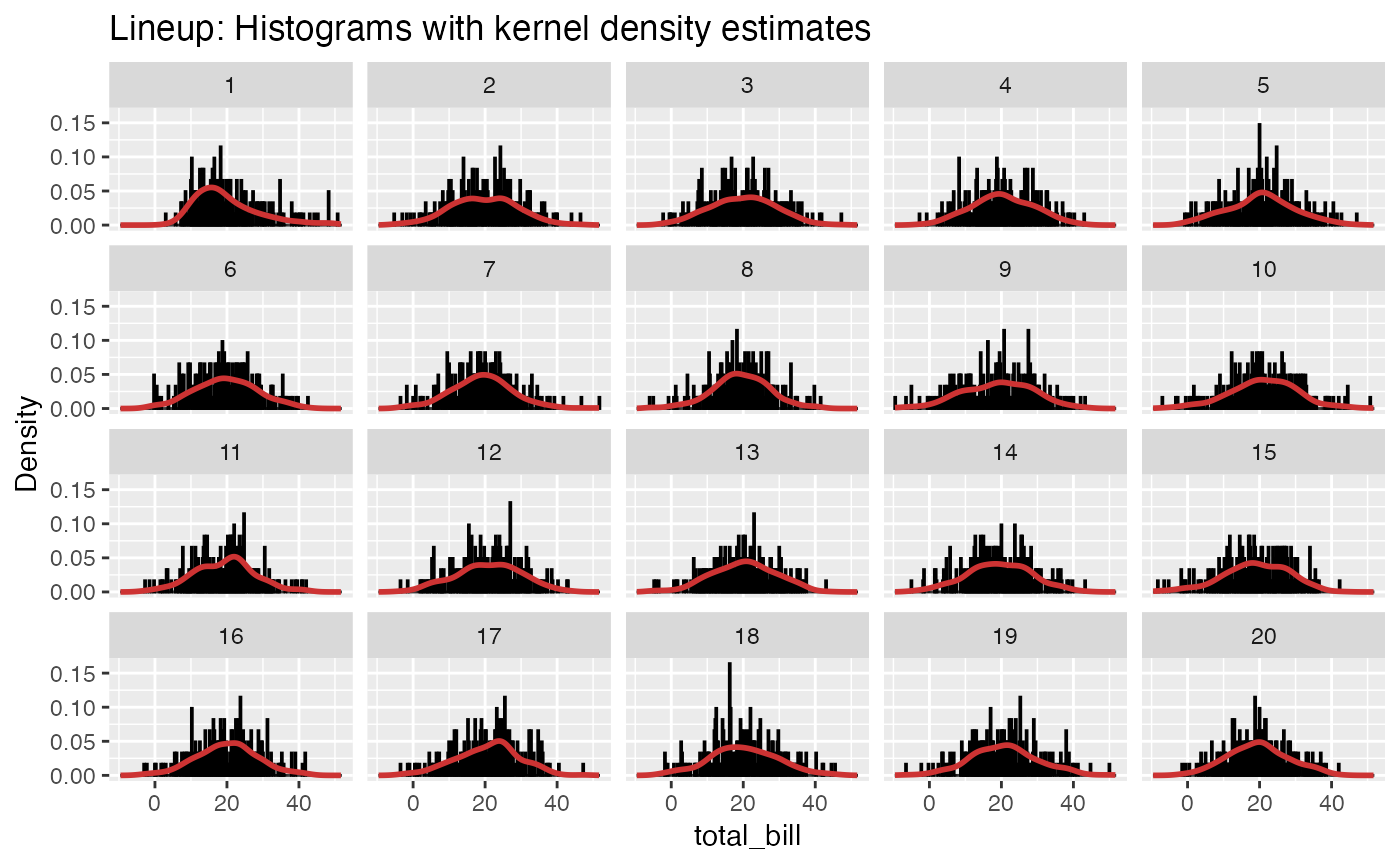
lineup_histograms(tips, "total_bill", dist = "normal") # Normal distribution
#> decrypt("DruT c2V2 AR LeOAVAeR JJ")

lineup_histograms(tips, "total_bill", dist = "gamma") # Gamma distribution
#> decrypt("DruT c2V2 AR LeOAVAeR JJ")


# Some distributions require that the parameters be specified:
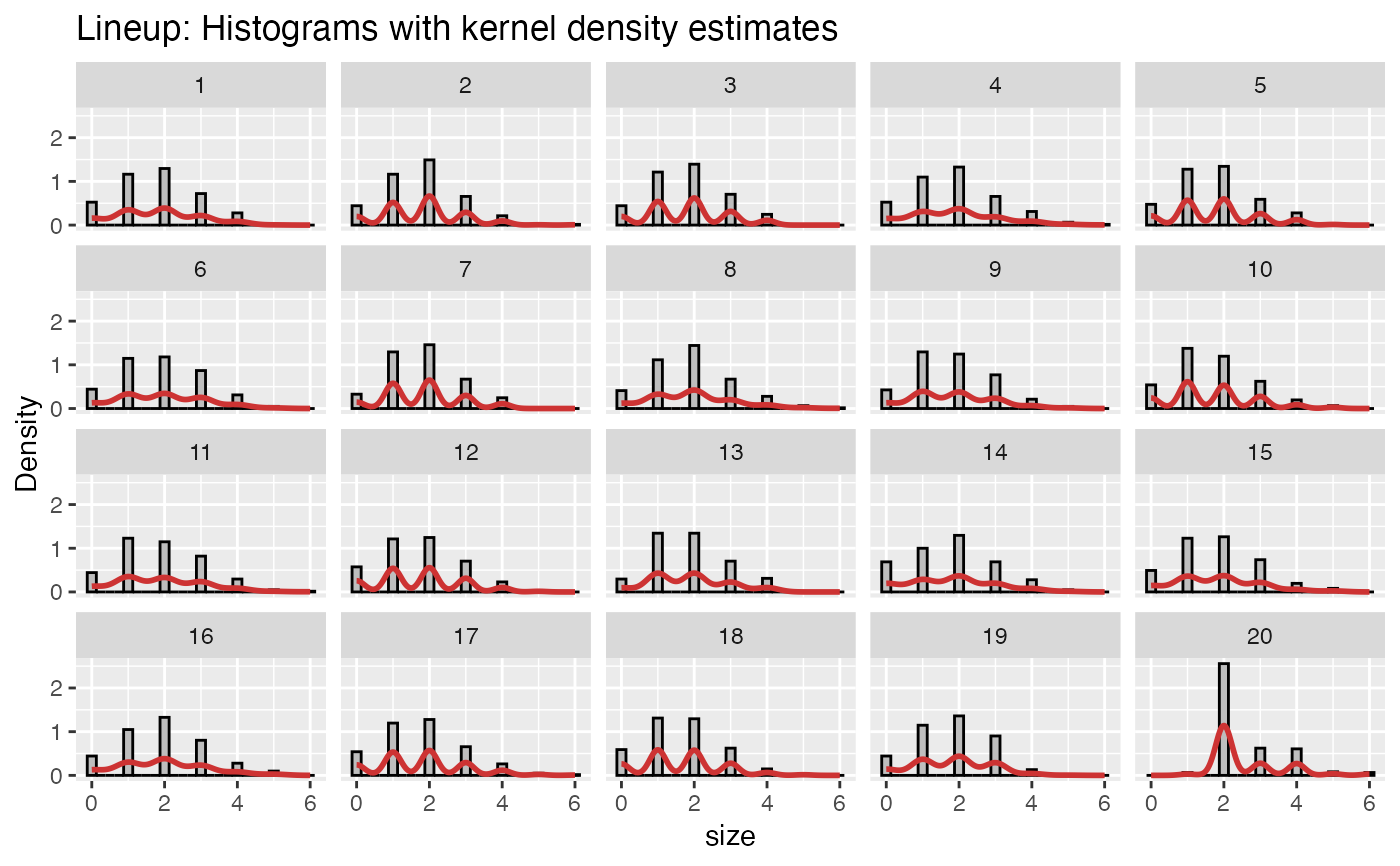
lineup_histograms(tips, "size", dist = "binomial", params = list(size = 6, p = 0.3))
#> decrypt("DruT c2V2 AR LeOAVAeR 1G")


# Style the plot using color settings and ggplot2 functions:
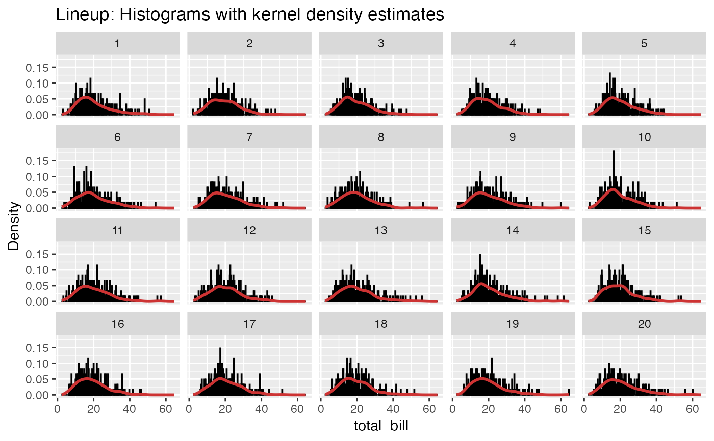
lineup_histograms(tips, "total_bill",
                  dist = "gamma",
                  color_bars = "steelblue",
                  color_lines = "magenta") +
    ggplot2::theme_minimal()
#> decrypt("DruT c2V2 AR LeOAVAeR Jz")